Learning Representations for Speech Recognition using Artificial

Learning Representations for Speech Recognition using Artificial Neural Networks

Paweł Świętojański

NI VER

S

E

R

G

O F

H

Y

TH

IT

E

U

D I U N B

Doctor of Philosophy Institute for Language, Cognition and Computation School of Informatics University of Edinburgh 2016

Lay Summary Learning representations is a central challenge in machine learning. For speech recognition, which concerns mapping speech acoustics into sequences of words, we are interested in learning robust representations that are stable across different acoustic environments, recording equipment and irrelevant inter– and intra– speaker variabilities. This thesis is concerned with representation learning for acoustic model adaptation to speakers and environments, construction of acoustic models in low-resource settings, and learning representations from multiple acoustic channels. The investigations are primarily focused on the hybrid approach to acoustic modelling based on hidden Markov models and artificial neural networks (ANN). The first contribution concerns acoustic model adaptation. This comprises two new adaptation transforms operating in ANN parameters space – Learning Hidden Unit Contributions (LHUC) and differentiable pooling. Both operate at the level of activation functions and treat a trained ANN acoustic model as a canonical set of fixed-basis functions, from which one can later derive variants tailored to the specific distribution present in adaptation data. On average, depending on the characteristics of the test set, 5-25% relative increase in accuracies were obtained in an unsupervised adaptation setting (scenario in which humanlevel manual transcriptions are not available). The second contribution concerns building acoustic models in low-resource data scenarios. In particular, we are concerned with insufficient amounts of transcribed acoustic material for estimating acoustic models in the target language. First we proposed an ANN with a structured output layer which models both context-dependent and context-independent speech units, with the contextindependent predictions used at runtime to aid the prediction of context-dependent units. We also propose to perform multi-task adaptation with a structured output layer. Those propositions lead to consistent accuracy improvements for both low-resource speaker-independent acoustic modelling and adaptation with LHUC technique. We then demonstrate that one can build better acoustic models with unsupervised multi– and cross– lingual initialisation and find that pre-training is a largely language-independent. Up to 14.4% relative accuracy improvements are observed, depending on the amount of the available transcribed acoustic data in the target language. i

The third contribution concerns building acoustic models from multi-channel acoustic data. For this purpose we investigate various ways of integrating and learning multi-channel representations. In particular, we investigate channel concatenation and the applicability of convolutional layers for this purpose. We propose a multi-channel convolutional layer with cross-channel pooling, which can be seen as a data-driven non-parametric auditory attention mechanism. We find that for unconstrained microphone arrays, our approach is able to match the performance of the comparable models trained on beamform-enhanced signals.

ii

Abstract Learning representations is a central challenge in machine learning. For speech recognition, we are interested in learning robust representations that are stable across different acoustic environments, recording equipment and irrelevant inter– and intra– speaker variabilities. This thesis is concerned with representation learning for acoustic model adaptation to speakers and environments, construction of acoustic models in low-resource settings, and learning representations from multiple acoustic channels. The investigations are primarily focused on the hybrid approach to acoustic modelling based on hidden Markov models and artificial neural networks (ANN). The first contribution concerns acoustic model adaptation. This comprises two new adaptation transforms operating in ANN parameters space. Both operate at the level of activation functions and treat a trained ANN acoustic model as a canonical set of fixed-basis functions, from which one can later derive variants tailored to the specific distribution present in adaptation data. The first technique, termed Learning Hidden Unit Contributions (LHUC), depends on learning distribution-dependent linear combination coefficients for hidden units. This technique is then extended to altering groups of hidden units with parametric and differentiable pooling operators. We found the proposed adaptation techniques pose many desirable properties: they are relatively low-dimensional, do not overfit and can work in both a supervised and an unsupervised manner. For LHUC we also present extensions to speaker adaptive training and environment factorisation. On average, depending on the characteristics of the test set, 5-25% relative word error rate (WERR) reductions are obtained in an unsupervised two-pass adaptation setting. The second contribution concerns building acoustic models in low-resource data scenarios. In particular, we are concerned with insufficient amounts of transcribed acoustic material for estimating acoustic models in the target language – thus assuming resources like lexicons or texts to estimate language models are available. First we proposed an ANN with a structured output layer which models both context–dependent and context–independent speech units, with the context-independent predictions used at runtime to aid the prediction of context-dependent states. We also propose to perform multi-task adaptation with a structured output layer. We obtain consistent WERR reductions up to iii

6.4% in low-resource speaker-independent acoustic modelling. Adapting those models in a multi-task manner with LHUC decreases WERRs by an additional 13.6%, compared to 12.7% for non multi-task LHUC. We then demonstrate that one can build better acoustic models with unsupervised multi– and cross– lingual initialisation and find that pre-training is a largely language-independent. Up to 14.4% WERR reductions are observed, depending on the amount of the available transcribed acoustic data in the target language. The third contribution concerns building acoustic models from multi-channel acoustic data. For this purpose we investigate various ways of integrating and learning multi-channel representations. In particular, we investigate channel concatenation and the applicability of convolutional layers for this purpose. We propose a multi-channel convolutional layer with cross-channel pooling, which can be seen as a data-driven non-parametric auditory attention mechanism. We find that for unconstrained microphone arrays, our approach is able to match the performance of the comparable models trained on beamform-enhanced signals.

iv

Acknowledgements I would like to express my gratitude to: • Steve Renals, for excellent supervision, patience, enthusiasm, scientific freedom and for the opportunity to pursue PhD studies in the Centre for Speech Technology Research (CSTR). It is hard to overstate how much I have benefited from Steve’s knowledge, expertise and advice. • My advisors: Peter Bell and Arnab Ghoshal, for engaging conversations and for many, much needed, suggestions during my PhD studies. Special thanks to Peter for proof-reading this dissertation. • My examiners: Hervé Bourlard, Simon King and Andrew Senior for peerreviewing this work and for the insightful comments which led to many improvements. All the shortcomings that remain are solely my fault. • Catherine Lai, for proof-reading parts of this thesis and Jonathan Kilgour for offering help with the AMI data preparation. Special thanks to Thomas Hain for useful feedback on distant speech recognition experiments, and for sharing components of the SpandH AMI setup with us. Thanks to Iain Murray and Hiroshi Shimodaira for the feedback during my annual reviews. • Everybody in the CSTR, for contributing towards a truly unique and superb academic environment. • The NST project (special thanks to Steve Renals (again!), Mark Gales, Thomas Hain, Simon King and Phil Woodland for making it happen). There were many excellent researchers working in NST, interacting with whom was a very rewarding experience. • Jinyu Li and Yifan Gong, for offering and hosting my two internships at Microsoft. Some of the ideas I developed there were used in this thesis. • Finally, I would like to say thanks to my family, for the constant and unfailing support and to Anna for incredible patience, understanding and encouragement over the last several years. This work was supported by EPSRC Programme Grant EP/I031022/1 Natural Speech Technology (NST). Thanks to the contributors of the Kaldi speech recognition toolkit and the Theano math expression compiler. v

Declaration I declare that this thesis was composed by myself, that the work contained herein is my own except where explicitly stated otherwise in the text, and that this work has not been submitted for any other degree or professional qualification except as specified.

(Paweł Świętojański)

vi

Table of Contents I

Preliminaries

2

1 Introduction

3

1.1

Thesis Structure . . . . . . . . . . . . . . . . . . . . . . . . . . . .

6

1.2

Declaration of content . . . . . . . . . . . . . . . . . . . . . . . .

6

1.3

Notation . . . . . . . . . . . . . . . . . . . . . . . . . . . . . . . .

9

2 Connectionist Models

12

2.1

Introduction . . . . . . . . . . . . . . . . . . . . . . . . . . . . . .

12

2.2

ANNs as a computational network . . . . . . . . . . . . . . . . . .

13

2.3

ANN components . . . . . . . . . . . . . . . . . . . . . . . . . . .

14

2.3.1

Loss functions . . . . . . . . . . . . . . . . . . . . . . . . .

14

2.3.2

Linear transformations . . . . . . . . . . . . . . . . . . . .

16

2.3.3

Activation functions . . . . . . . . . . . . . . . . . . . . .

17

2.4

Training . . . . . . . . . . . . . . . . . . . . . . . . . . . . . . . .

19

2.5

Regularisation . . . . . . . . . . . . . . . . . . . . . . . . . . . . .

20

2.6

Summary . . . . . . . . . . . . . . . . . . . . . . . . . . . . . . .

20

3 Overview of Automatic Speech Recognition

21

3.1

Brief historical outlook . . . . . . . . . . . . . . . . . . . . . . . .

21

3.2

Introduction to data-driven speech recognition . . . . . . . . . . .

23

3.3

Hidden Markov acoustic models . . . . . . . . . . . . . . . . . . .

25

3.3.1

HMM assumptions . . . . . . . . . . . . . . . . . . . . . .

26

3.3.2

On the acoustic units and HMM states . . . . . . . . . . .

27

3.3.3

Modelling state probability distributions in HMMs . . . .

28

3.3.4

Estimating parameters of HMM-based acoustic model . . .

32

3.4

Language model . . . . . . . . . . . . . . . . . . . . . . . . . . . .

34

3.5

Feature extraction

35

. . . . . . . . . . . . . . . . . . . . . . . . . .

vii

3.5.1

ANNs as feature extractors

. . . . . . . . . . . . . . . . .

36

3.6

Decoding . . . . . . . . . . . . . . . . . . . . . . . . . . . . . . . .

37

3.7

Evaluation . . . . . . . . . . . . . . . . . . . . . . . . . . . . . . .

38

3.8

Summary . . . . . . . . . . . . . . . . . . . . . . . . . . . . . . .

38

4 Corpora and Baseline Systems 4.1

Introduction . . . . . . . . . . . . . . . . . . . . . . . . . . . . . .

39

4.2

TED Lectures . . . . . . . . . . . . . . . . . . . . . . . . . . . . .

40

4.2.1

Language models . . . . . . . . . . . . . . . . . . . . . . .

42

AMI and ICSI meetings corpora . . . . . . . . . . . . . . . . . . .

42

4.3.1

AMI . . . . . . . . . . . . . . . . . . . . . . . . . . . . . .

42

4.3.2

ICSI . . . . . . . . . . . . . . . . . . . . . . . . . . . . . .

43

4.3.3

Acoustic models . . . . . . . . . . . . . . . . . . . . . . . .

44

4.3.4

Lexicon and language model . . . . . . . . . . . . . . . . .

45

4.4

Switchboard . . . . . . . . . . . . . . . . . . . . . . . . . . . . . .

45

4.5

Aurora4 . . . . . . . . . . . . . . . . . . . . . . . . . . . . . . . .

46

4.6

GlobalPhone multi-lingual corpus . . . . . . . . . . . . . . . . . .

47

4.7

Notes on statistical significance tests . . . . . . . . . . . . . . . .

48

4.3

II

39

Adaptation and Factorisation

51

5 Learning Hidden Unit Contributions

52

5.1

Introduction . . . . . . . . . . . . . . . . . . . . . . . . . . . . . .

52

5.2

Review of Neural Network Acoustic Adaptation . . . . . . . . . .

53

5.3

Learning Hidden Unit Contributions (LHUC) . . . . . . . . . . .

56

5.4

Speaker Adaptive Training LHUC (SAT-LHUC) . . . . . . . . . .

60

5.5

Results . . . . . . . . . . . . . . . . . . . . . . . . . . . . . . . . .

64

5.5.1

LHUC hyperparameters . . . . . . . . . . . . . . . . . . .

64

5.5.2

SAT-LHUC . . . . . . . . . . . . . . . . . . . . . . . . . .

65

5.5.3

Sequence model adaptation . . . . . . . . . . . . . . . . .

72

5.5.4

Other aspects of adaptation . . . . . . . . . . . . . . . . .

74

5.5.5

Complementarity to feature normalisation . . . . . . . . .

78

5.5.6

Adaptation Summary . . . . . . . . . . . . . . . . . . . . .

79

5.6

LHUC for Factorisation

. . . . . . . . . . . . . . . . . . . . . . .

82

5.7

Summary . . . . . . . . . . . . . . . . . . . . . . . . . . . . . . .

85

viii

6 Differentiable Pooling

88

6.1

Introduction . . . . . . . . . . . . . . . . . . . . . . . . . . . . . .

88

6.2

Differentiable Pooling . . . . . . . . . . . . . . . . . . . . . . . . .

89

6.2.1

Lp -norm (Diff-Lp ) pooling . . . . . . . . . . . . . . . . .

91

6.2.2

Gaussian kernel (Diff-Gauss) pooling . . . . . . . . . . .

91

Learning Differentiable Poolers . . . . . . . . . . . . . . . . . . .

92

6.3.1

Learning and adapting Diff-Lp pooling . . . . . . . . . .

92

6.3.2

Learning and adapting Diff-Gauss pooling regions . . . .

93

6.4

Representational efficiency of pooling units . . . . . . . . . . . . .

96

6.5

Results . . . . . . . . . . . . . . . . . . . . . . . . . . . . . . . . .

97

6.5.1

Baseline speaker independent models . . . . . . . . . . . .

97

6.5.2

Adaptation experiments . . . . . . . . . . . . . . . . . . . 100

6.3

6.6

III

Summary and Discussion . . . . . . . . . . . . . . . . . . . . . . . 109

Low-resource Acoustic Modelling

7 Multi-task Acoustic Modelling and Adaptation

113 114

7.1

Introduction . . . . . . . . . . . . . . . . . . . . . . . . . . . . . . 114

7.2

Structured Output Layer . . . . . . . . . . . . . . . . . . . . . . . 115

7.3

Experiments . . . . . . . . . . . . . . . . . . . . . . . . . . . . . . 119

7.4

7.3.1

Structured output layer

. . . . . . . . . . . . . . . . . . . 120

7.3.2

Multi-task adaptation . . . . . . . . . . . . . . . . . . . . 122

7.3.3

Full TED and Switchboard . . . . . . . . . . . . . . . . . . 123

Summary . . . . . . . . . . . . . . . . . . . . . . . . . . . . . . . 125

8 Unsupervised multi-lingual knowledge transfer

126

8.1

Introduction . . . . . . . . . . . . . . . . . . . . . . . . . . . . . . 126

8.2

Review of low-resource acoustic modelling . . . . . . . . . . . . . 127

8.3

ANNs and restricted Boltzmann machines . . . . . . . . . . . . . 129

8.4

Experiments . . . . . . . . . . . . . . . . . . . . . . . . . . . . . . 130

8.5

8.4.1

Baseline results . . . . . . . . . . . . . . . . . . . . . . . . 130

8.4.2

ANN configuration and results . . . . . . . . . . . . . . . . 131


ix

IV

Distant Speech Recognition

9 Learning Representations from Multiple Acoustic Channels

140 141

9.1

Introduction . . . . . . . . . . . . . . . . . . . . . . . . . . . . . . 141

9.2

Review of DSR approaches . . . . . . . . . . . . . . . . . . . . . . 142

9.3

Learning representation from multiple channels . . . . . . . . . . 144

9.4

9.5

9.6

9.3.1

Beamforming . . . . . . . . . . . . . . . . . . . . . . . . . 144

9.3.2

Channel concatenation . . . . . . . . . . . . . . . . . . . . 145

9.3.3

Convolutional and pooling layers . . . . . . . . . . . . . . 147

Experiments (I) . . . . . . . . . . . . . . . . . . . . . . . . . . . . 150 9.4.1

Baseline results . . . . . . . . . . . . . . . . . . . . . . . . 150

9.4.2

Channel concatenation and data pooling . . . . . . . . . . 153

9.4.3

Convolutional Neural Networks . . . . . . . . . . . . . . . 154

9.4.4

SDM – Single Distant Microphone . . . . . . . . . . . . . . 154

9.4.5

MDM – Multiple Distant Microphones . . . . . . . . . . . 155

Experiments (II) . . . . . . . . . . . . . . . . . . . . . . . . . . . 156 9.5.1

SDM – Single Distant Microphone . . . . . . . . . . . . . . 157

9.5.2

MDM – Multiple Distant Microphones . . . . . . . . . . . 158

9.5.3

IHM – Individual Headset Microphone . . . . . . . . . . . 159


10 Conclusions

162

10.1 Overview of contributions . . . . . . . . . . . . . . . . . . . . . . 162 10.2 Further work . . . . . . . . . . . . . . . . . . . . . . . . . . . . . 165 Bibliography

167

x

TABLE OF CONTENTS

1

Part I Preliminaries

2

Chapter 1 Introduction This thesis concerns learning and adapting representations for acoustic modelling in automatic speech recognition (ASR). We are primarily concerned with hidden Markov-based acoustic models [Baker, 1975] in which state probability distributions are estimated by connectionist architectures [Rosenblatt, 1962]. This is sometimes referred to as the hybrid approach to ASR first proposed by [Bourlard and Wellekens, 1990, Bourlard and Morgan, 1990], intensively developed in mid nineties [Bourlard et al., 1992, Renals et al., 1994, Bourlard and Morgan, 1994], and more recently refined to give state of the art results on multiple speech recognition benchmarks by Hinton et al. [2012] and many others. Representation learning [Rumelhart et al., 1986] reflects a shift from a knowledgebased towards a data-driven means of extracting useful features from data. This process typically involves building multiple-levels of transformations jointly with a target predictor, driven by a single task-related objective. It is still possible to incorporate knowledge-motivated priors and assumptions; however, they tend to be much more generic when compared to the expertise engineered in handcrafted features where one usually seeks for representation adjusted for strengths and weaknesses of the specific classifier. Connectionist architectures have been very successful in representation learning in both supervised and unsupervised settings [Bengio et al., 2013]. This is not surprising and to a large degree may be attributed to gradient-based iterative learning algorithms [Rumelhart et al., 1986], which work well in practice. In addition, they provide modelling power which, under some mild assumptions, has been proved to be a universal approximator for smooth functions [Cybenko, 1989, Hornik et al., 1989, Barron, 1993]. Notice, however, that the universal approxi3

Chapter 1. Introduction

4

mation theorem says little about how to make use of those theoretical properties in practice or even how to relate the optimal model capacity to the given data. Nevertheless, ANNs offer an appealing unified framework for learning representations, allowing a focus on more generic aspects – for example, how to design an appropriate loss functions for the task or designing an optimiser capable of searching for model parameters which minimise this loss. At the same time ANNs give some guarantee that the model’s parametrisation will have a sufficient capacity1 to learn a satisfactory solution without worrying whether data fits predictor’s capabilities. We will elaborate on this brief outline later in Chapter 2. Despite significant progress in acoustic model development over the last several decades, including recent work on ANNs, ASR systems remain strongly domain dependent requiring specific task-oriented systems for good performance. Furthermore, it has been found that properly performed normalisation of the acoustic feature-space or direct adaptation of acoustic model parameters in a speaker-dependent manner yields significant gains in accuracy. This lack of generality is particularly pronounced for far-field speech recognition – in this case, the available corpora allow for controlled experiments marginalising the impact of all but the acoustic component on the final system performance to be carried out. The results show that extending the distance at which the speech is captured can double error rates – and this already assumes a matched scenario with two sets of independently trained models, one for distant and one for close-talking data. This thesis is concerned with three major themes: 1. Adapting representations: We are primarily concerned with adaptation techniques operating in the parameter space of an ANN. In particular, we have developed a technique that relies on learning hidden unit contributions (LHUC) [Swietojanski and Renals, 2014] and offers a principled interpretation rooted in the universal approximation theorem. Building on LHUC we have extended it to a speaker-adaptive training variant able to work both in speaker independent and dependent manners [Swietojanski and Renals, 2016]. The work on LHUC took us towards related techniques that rely on differentiable pooling operators, in which adaptation is carried by estimating speaker-specific pooling regions [Swietojanski and Renals, 2015]. Within this avenue we focused on two types of pooling parametrisations - Lp and Gaussian weighted units. Both approaches were thoroughly 1

In a sense that the number of model’s parameters can be easily increased if necessary.


5

examined experimentally on multiple large vocabulary speech recognition (ASR) benchmarks. Results and broader motivations of those were reported in [Swietojanski, Li, and Renals, 2016] and [Swietojanski and Renals, 2016]. 2. Learning representations under low-resource acoustic conditions: Adapting context-dependent models with small amounts of data results in very sparsely distributed adaptation targets – resulting in updating of only few outputs. To compensate for this we propose a multi-task adaptation with a structured output layer using an auxiliary context-independent layer to adapt context-dependent targets [Swietojanski, Bell, and Renals, 2015]. This structure also help in the generic scenario of speaker-independent lowsource acoustic modelling. It is sometimes difficult to access transcribed data for some languages. As a result ASR systems in such scenarios offer much lower accuracy compared to similar systems estimated for resources-rich languages. Within this part we try to leverage multi-lingual acoustic data to improve ASR for a target under-resourced language. In particular, we propose unsupervised multilingual pre-training as a form of multi-lingual knowledge transfer [Swietojanski, Ghoshal, and Renals, 2012]. 3. Learning representations from multiple channels: Much work has been done in multi-microphone acoustic modelling employing conventional Gaussian mixture models. The consensus found in the literature is that optimal performance involves beamforming of multiple-channels in order to create a single but enhanced audio signal. ANNs offer a very flexible framework to combine various sources of information and in Chapter 9 we investigate their applicability to model-based learning from multiple acoustic channels. In particular, we investigate different ways of combining multi-channel data in the model [Swietojanski, Ghoshal, and Renals, 2013a] and propose a convolutional layer with two-levels of pooling [Swietojanski, Ghoshal, and Renals, 2014a]. This approach, for unconstrained microphones, is able to match models trained on signal-enhanced speech [Renals and Swietojanski, 2014]. A side result of this work is the creation of publicly available recipes for the AMI and ICSI meeting corpora released with the Kaldi speech recognition toolkit (www.kaldi-asr.org).


1.1

6

Thesis Structure

Given above contributions, the thesis is organised as follows: Chapter 2 provides a short introduction to connectionist models. Chapter 3 contains a brief and high level review of large vocabulary speech recognition. Chapter 4 gathers together descriptions and statistics of the corpora used to carry out the experiments. We follow an in-place approach in this work – we present experimental results in each chapter following theoretical descriptions. Chapter 5 reviews adaptation methods and introduces Learning Hidden Unit Contributions (LHUC) and its speaker adaptively trained (SAT) variant. Chapter 6 continues the adaptation topic and presents model-based adaptation using parametric and differentiable pooling operators. Chapter 7 investigates low-resource acoustic models and adaptation using a multi-task training and adaptation with structured output layer. Chapter 8 concerns unsupervised multi-lingual knowledge transfer. Chapter 9 investigates the use of multiple channels in distant speech recognition, where our primary focus lies in explicit representation learning from multichannel acoustic data. Chapter 10 contains a summary and discusses possible future work.

1.2

Declaration of content

This thesis is almost completely composed of the work published in the following journal and conference papers: • P. Swietojanski and S. Renals. Differentiable Pooling for Unsupervised Acoustic Model Adaptation. IEEE/ACM Transactions on Audio, Speech and Language Processing, 2016 • P. Swietojanski J. Li and S. Renals. Learning Hidden Unit Contributions for Unsupervised Acoustic Model Adaptation. IEEE/ACM Transactions on Audio, Speech and Language Processing, 2016 • P. Swietojanski and S. Renals. SAT-LHUC: Speaker Adaptive Training for Learning Hidden Unit Contributions. In Proc. IEEE International Con-


7

ference on Acoustics, Speech and Signal Processing (ICASSP), Shanghai, China, 2016 • P. Swietojanski, P. Bell, and S. Renals. Structured output layer with auxiliary targets for context-dependent acoustic modelling. In Proc. ISCA Interspeech, Dresden, Germany, 2015. • P. Swietojanski and S. Renals. Differentiable pooling for unsupervised speaker adaptation. In Proc. IEEE International Conference on Acoustics, Speech and Signal Processing (ICASSP), Brisbane, Australia, 2015 • P. Swietojanski and S. Renals. Learning hidden unit contributions for unsupervised speaker adaptation of neural network acoustic models. In Proc. IEEE Spoken Language Technology Workshop (SLT), Lake Tahoe, USA, 2014 • P. Swietojanski, A. Ghoshal, and S. Renals. Convolutional neural networks for distant speech recognition. IEEE Signal Processing Letters, 21(9):11201124, September 2014 • S. Renals and P. Swietojanski. Neural networks for distant speech recognition. In The 4th Joint Workshop on Hands-free Speech Communication and Microphone Arrays (HSCMA), Nancy, France, 2014 • P. Swietojanski, A. Ghoshal, and S. Renals. Hybrid acoustic models for distant and multichannel large vocabulary speech recognition. In Proc. IEEE Automatic Speech Recognition and Understanding Workshop (ASRU), Olomouc, Czech Republic, 2013 • P. Swietojanski, A. Ghoshal, and S. Renals. Unsupervised cross-lingual knowledge transfer in DNN-based LVCSR. In Proc. IEEE Spoken Language Technology Workshop (SLT), pages 246-251, Miami, Florida, USA, 2012. Some related aspects in the thesis were inspired, but did not get into directly, by the following work I have (co-)authored: • P. Swietojanski, J-T Huang and J. Li. Investigation of maxout networks for speech recognition. In Proc. IEEE International Conference on Acoustics, Speech and Signal Processing (ICASSP), Florence, Italy, 2014


8

• P. Swietojanski, A. Ghoshal, and S. Renals. Revisiting hybrid and GMMHMM system combination techniques. In Proc. IEEE International Conference on Acoustics, Speech and Signal Processing (ICASSP), Vancouver, Canada, 2013 • P. Bell, P. Swietojanski, and S. Renals. Multi-level adaptive networks in tandem and hybrid ASR systems. In Proc. IEEE International Conference on Acoustics, Speech and Signal Processing (ICASSP), Vancouver, Canada, 2013 • A. Ghoshal, P. Swietojanski, and S. Renals. Multilingual training of deep neural networks. In Proc. IEEE International Conference on Acoustics, Speech and Signal Processing (ICASSP), Vancouver, Canada, 2013 Beyond above works, during my PhD days I also had a chance to contribute towards related research projects and speech recognition evaluations (IWSLT12, IWSLT14 and MGB Challenge 2015), some of those collaborations resulted in peer-reviewed publications, as follows: • Z. Wu, P. Swietojanski, C. Veaux, S. Renals, and S. King. A study of speaker adaptation for DNN-based speech synthesis. In Proc. ISCA Interspeech, Dresden, Germany, 2015 • P. Bell, P. Swietojanski, J. Driesen, Mark Sinclair, Fergus McInnes, and Steve Renals. The UEDIN ASR systems for the IWSLT 2014 evaluation. In Proc. International Workshop on Spoken Language Translation (IWSLT), South Lake Tahoe, USA, 2014 • P. Bell, H. Yamamoto, P. Swietojanski, Y. Wu, F. McInnes, C. Hori, and S. Renals. A lecture transcription system combining neural network acoustic and language models. In Proc. ISCA Interspeech, Lyon, France, 2013 • H. Christensen, M. Aniol, P. Bell, P. Green, T. Hain, S. King, and P. Swietojanski. Combining in-domain and out-of-domain speech data for automatic recognition of disordered speech. In Proc. ISCA Interspeech, Lyon, France, 2013 • P. Lanchantin, P. Bell, M. Gales, T. Hain, X. Liu, Y. Long, J. Quinnell, S. Renals, O. Saz, M. Seigel, P. Swietojanski, and P. Woodland. Automatic


9

transcription of multi-genre media archives. In Proc. Workshop on Speech, Language and Audio in Multimedia, Marseille, France, 2013 • P. Bell, M. Gales, P. Lanchantin, X. Liu, Y. Long, S. Renals, P. Swietojanski, and P. Woodland. Transcription of multi-genre media archives using out-of-domain data. In Proc. IEEE Spoken Language Technology Workshop (SLT), pages 324-329, Miami, Florida, USA, 2012 • E. Hasler, P. Bell, A. Ghoshal, B. Haddow, P. Koehn, F. McInnes, S. Renals, and P. Swietojanski. The UEDIN system for the IWSLT 2012 evaluation. In Proc. International Workshop on Spoken Language Translation (IWSLT), Hong Kong, China, 2012

1.3

Notation

The following notation has been used throughout this work. ot

speech observation at time t

ort

the “static” elements of feature vector ot

∆ort

the “delta” elements of feature vector ot

∆2 ort ¯t O

the “delta-delta” elements of feature vector ot context window of 2c + 1 speech observations: ¯ t = [o> , . . . , o> , . . . , o> ]> O t−c

t

t+c

O1:T

observation sequence o1 , . . . , oT

θ

an arbitrary set of parameters

F(θ)

a criterion to be optimised over parameters θ

f (x; θ)

an arbitrary neural network, parametrised by θ, acting on input x

f l (x; θ l )

lth layer of neural network, parametrised by θ l

Wl

weight matrix associated with layer l of a neural network

wil

weight vector associated with node i for layer l

bl

bias vector at lth layer

l

φ (·)

non-linear function applied at lth layer

hl

vector of hidden activations at lth layer

cm

the prior of Gaussian component m

µ(m)

the mean of Gaussian component m


10

Σ(m)

the covariance matrix of Gaussian component m

N (µ, Σ)

Gaussian distribution with mean µ and covariance matrix Σ

N (ot ; µ, Σ)

likelihood of observation ot being generated by N (µ, Σ)

p(O1:T ; θ)

likelihood of observation sequence O1:T given parameters θ

qj

state j of the HMM

Q

the HMM state sequence q1:T

Q

set of all HMM states

A

an arbitrary transformation matrix

A>

transpose of A

A−1

inverse of A

|A|

determinant of A

aij

element i, j of A

Acronyms ANN

artificial neural network

BMMI

boosted maximum mutual information

ASR

automatic speech recognition

CMN

cepstral mean normalisation

CMLLR

constrained maximum likelihood linear regression

CNN

ANN with at least one convolutional layer

CVN

cepstral variance normalisation

DNN

(deep) artificial neural network (the same as ANN)

EM

expectation maximisation

EBP

error back-propagation

FBANK

log mel filterbank

FFT

fast Fourier transform

GMM

Gaussian mixture model

HMM

hidden Markov model

LVCSR

large vocabulary continuous speech recognition

LDA

linear discriminant analysis

Chapter 1. Introduction LHUC

learning hidden unit contributions

LM

language model

MBR

minimum Bayes risk

MFCC

mel-frequency cepstral coefficients

ML

maximum likelihood

MLLR

maximum likelihood linear regression

MLLT

maximum likelihood linear transform

MMI

maximum mutual information

MMSE

minimum mean square error

PLP

perceptual linear prediction

PPL

perplexity of a language model

PDF

probability density function

RBM

restricted Boltzmann machine

RNN

recurrent neural network

SAT

speaker adaptive training

SOL

structured output layer

SD

speaker dependent parameters

SI

speaker independent parameters

SNR

signal to noise ratio

TDOA

time delay of arrival

VTLN

vocal tract length normalisation

WER

word error rate

11

Chapter 2 Connectionist Models This chapter presents the background on the construction and learning of artificial neural network models.

2.1

Introduction

The concept of connectionism dates back as far as 400 B.C. and Aristotle’s notion of mental association [Medler, 1998] and has been since influenced by many fields of science and philosophy, as outlined in the survey by Medler [1998]. In this thesis we are interested in the “post-perceptron” era of connectionism, or an engineering approach, especially in the context of the distributed parallel processing framework proposed by [Rumelhart et al., 1986] and the definition given in Bourlard and Morgan [1994] which describes a connectionist system as a: System in which information is represented and processed in terms of the input pattern and strength of connections between units that do some simple processing on their input. In the literature, connectionist systems are often referred to as {artificial, multi-layer, deep} neural networks or multi-layer perceptrons. Hereafter in this thesis we will primarily rely on feed-forward structures and we will use term artificial neural network (ANN) when referring to such models, where necessary we will also explicitly specify the type of connectivity pattern of its parameters (feed-forward, recurrent, convolutional, or a combination of those).

12

Chapter 2. Connectionist Models

2.2

13

ANNs as a computational network

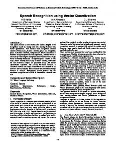
A convenient way to explain the computations performed by an arbitrary connectionist model is by treating the computation as traversing and executing a series of computational nodes organised in a graph [LeCun et al., 1998a]. Denote by G = {V, E} a graph consisting of a set of vertices (or nodes) V and a set of connecting edges (or links) E. Such a graph must exhibit certain properties: i) its edges should be directed, thus defining one-directional dependencies between vertices V and ii) paths defined by edges (possibly spanning many vertices) must not create cycles, given a specified dependency structure. This is a non-rigorous definition of a Directed Acyclic Graph (DAG). Figure 2.1 (a) depicts an illustration of such a DAG with four vertices V = {A, B, C, D}, each of those vertices as well as the whole block computes a function Y from inputs X using parameters θ. The dependency structure allows us to easily find the order in which one need to execute the operations – this is known as a topological ordering and can be obtained by traversing the graph in depthfirst order, starting from its inputs (root). Assuming we know how to perform computations at each node, following this topological ordering and evaluating visited nodes will effectively perform the forward-pass procedure. In a similar way, starting from the forward computation DAG, one can build a similar DAG whose traversal will result in the error back-propagation procedure [Rumelhart et al., 1986], as illustrated in Figure 2.1 (b).

Figure 2.1: (Left) Computational graph consisting of some 4 internal computations, A, B, C and D parametrised by a, b, c and d, respectively. (Right) corresponding back-propagation graph


14

Typically, each computational node is required to implement three types of computations: • Forward computation through the node, • Backward computation: gradient of the outputs of the node with respect to its inputs, • Gradient of the outputs of the node with respect to its parameters (if any) The loss function, used to guide the learning process, can also be represented as a node with two inputs (targets, model predictions) and a scalar output representing cost which allows DAG representations of arbitrary learnable ANN structures, as long as each component knows how to perform the forward and backward computations. Examples presented hitherto underline some generic principles allowing us to build arbitrarily complex computational graphs keeping the underlying computational machinery the same. In the next section, we outline some of the typical choices for such nodes, divided into three categories: loss functions, linear transforms and activation functions.

2.3

ANN components

A feed-forward ANN is implemented as a nested function comprising of L processing layers, parametrised by θ, which maps some input x into output y:

f (x; θ) = f L f L−1 . . . f 2 f 1 x; θ 1 ; θ 2 . . . ; θ L−1 ; θ L

(2.1)

The particular mapping that an ANN can learn will depend on the type of connectivity pattern and hidden activation function in each layer, and the type of output layer activation and the loss function. We review them briefly below.

2.3.1

Loss functions

In order to learn the parameters of an ANN, we must specify a suitable loss function. The loss function, to be minimised, does not necessarily need to be easy to evaluate, as long as one can compute its gradient or provide a satisfactory approximation to it. Below we list some of the popular choices that often also


15

act as surrogate loss functions for the tasks in which more suitable losses are not available. Let y be the output layer activations produced by a neural network f (x; θ) and let t denote training targets for a given task, then we have: • Squared Errors: A suitable loss for regression tasks when the target t contain real numbers and f (x; θ) produces linear activations: 1 FSE (t, y) = ||t − y||2 2

(2.2)

∂FSE (t, y) =y−t ∂y

(2.3)

• Cross-entropy: in cases where both t and y are categorical probability distributions (i.e. for any valid output i, 0 < yi < 1 and

P

i

yi = 1). It is

suitable to minimise the Kullback-Leibler divergence of y from t: X ti KL(t||y) = ti log yi i =

X

ti log ti −

i

X

ti log yi

(2.4) (2.5)

i

Since the parameters θ of an ANN f (x; θ) used to produce y do not depend on the first part of (2.5) the loss to minimise, and its gradient with respect to y are: FCE (t, y) = −

X

ti log yi

(2.6)

i

ti ∂FCE (ti , yi ) =− ∂yi yi

(2.7)

• Binary cross-entropy is a special case of cross-entropy when there are only two classes or in scenarios in which activations at the output layer are probabilistic but independent from each other, in which case the loss and its gradient with respect to y is: FBCE (t, y) = −t log y − (1 − t) log(1 − y)

(2.8)

∂FCE (t, y) t 1−t =− + ∂y y 1−y

(2.9)

• Other: Ideally one would like to optimise the loss which directly corresponds to the performance metric of the task at hand. For example in speech transcription, where one is interested in optimising sequential performance, customised loss functions may yield improved performance [Povey, 2003, Kingsbury, 2009] (see also Section 3.3.4).


2.3.2

16

Linear transformations

In this section we describe two types of linear transformations commonly used with ANN in fully-connected and convolutional settings. • Affine transform: implements a dot product and a shift: a = W> x + b

(2.10)

by taking a derivatives w.r.t the input (x) and the transform parameters (θ = {W, b}) we have: ∂a = W, ∂x

∂a = x, ∂W

∂a =1 ∂b

(2.11)

• Affine transform with convolution: implements a local connectivity pattern which is typically shared across multiple locations in the layer’s input space [LeCun and Bengio, 1995]. Typically, with ANNs we perform convolution along one, two or three dimensions. In particular, in this thesis we use one dimensional convolution along the frequency axis as in [AbdelHamid et al., 2014], in which case the k-th convolutional filter (out of total J such filters in a layer) can be expressed as a dot product1 . Denote by x = [x1 , x2 , . . . , xM ]> some M -dimensional input signal and by k > ] the weights of the kth N-dimensional convolutional wk = [w1k , w2k , . . . , wN

filter. Then one can build a large but sparse matrix Wk by replicating wk filters as in (2.12) and then computing the convolutional linear activations for each of J filters as in (2.10). 

k wk w2k . . . wN  1

Wk> =

         

0

w1k w2k

0

k . . . wN

0 .. .

0 .. .

w1k ...

w2k ...

0

0

...

0

0

...

0

...

k . . . wN ... ... ... ...

w1k

w2k



0   0   0 .. .

k . . . wN

      

(2.12)

Extra steps must be taken when computing the gradients with respect to parameters, in which case one needs to take into account the fact the kth kernel wk is shared across many locations, and the total gradient is the sum of the intermediate gradients computed with wk at multiple locations in x. 1

One does not need to flip the filter index (in order to perform convolution in the mathematical sense) as the filters are data-driven and the same result can be obtained using crosscorrelation instead, which is more efficient computationally.


2.3.3

17

Activation functions

Linear transformations are usually followed by non-linear activation functions. Those functions can either act element-wise or take into account groups of units. Assuming a is the vector of linear activations obtained with (2.10) and ai is its ith element, popular choices for non-linear functions are as follows: • Identity: results in no transformation of linear activations in (2.10). These are typically used in the output layer for regression tasks, but also at hidden layers with bottle-neck feature extractors and as an adaptation transform. φ(ai ) = ai

(2.13)

• Sigmoid: squashing non-linearity resulting in activations bounded by [0, 1]: φ(ai ) =

1 1 + exp(−ai )

∂φ(ai ) = φ(ai )(1 − φ(ai )) ∂ai

(2.14)

(2.15)

• Hyperbolic tangent (tanh): squashing non-linearity resulting in activations bounded by [−1, 1]: φ(ai ) =

exp(ai ) − exp(−ai ) exp(ai ) + exp(−ai )

∂φ(ai ) = 1 − φ(ai )2 ∂ai

(2.16)

(2.17)

• Rectified Linear Unit (ReLU) [Nair and Hinton, 2010]: ReLU implements a form of data-driven sparsity – on average the activations are sparse, but the general sparsity pattern will depend on particular data-point. This is different from the sparsity obtained in parameters space with L1 regularisation (see also Section 2.5) as the latter affects all data-points in the same way. Given a linear activation ai , ReLU forward and backward computations are given as follows: φ(ai ) = max(0, ai ),   1

∂φ(ai ) =  ∂ai  0

if ai > 0 if ai < 0

(2.18)

(2.19)


18

• Maxout (or max-pooling in general) [Riesenhuber and Poggio, 1999, Goodfellow et al., 2013]: maxout is an example of a type of data-driven nonlinearity in which the transfer function can be learned from data – the model can build a non-linear activation from piecewise linear components. These linear components, depending on the number of linear regions used in the pooling operator, can approximate other functions, such as ReLU or absolute value. Given some set {ai }i∈R of R linear activations, maxout implements the following operation: φ({ai }i∈R ) = max({ai }i∈R )   1

∂φ({ai }i∈R ) =  ∂ai∈R 0

if ai is the max activation

(2.20)

(2.21)

otherwise

• Lp –norm [Boureau et al., 2010]: the activation is implemented as an L-norm with an arbitrary order p ≥ 1 (in order to satisfy triangle inequality, see also Chapter 6) over a set {ai }i∈R of R linear activations: !1

p

φ({ai }i∈R ) =

X

p

|ai |

(2.22)

i∈R

ai · |ai |p−2 ∂φ({ai }i∈R ) =P · φ({ai }i∈R ) p ∂ai∈R j∈R |aj |

(2.23)

• Softmax [Bridle, 1990]: To obtain a probability distribution one can use the softmax non-linearity (2.24) which is a generalisation of sigmoid activations to multi-class problems. Softmax operation is prone to both over– and under–flows. Over-flows are typically addressed by subtracting the maximum activation m = max(a) before evaluating exponentials, as in the rightmost part of (2.24). If necessary, under–flows can be avoided with applying the same trick and computing the logarithm of softmax instead. exp(ai − m) exp(ai ) =P φ(ai ) = P j exp(aj ) j exp(aj − m)

(2.24)

The derivative of softmax with respect to linear activation is given in (2.25), where δij is the Kronecker delta function: φ(ai ) = φ(ai )(δij − φ(aj )) aj

(2.25)


2.4

19

Training

Most techniques for estimating ANN parameters are gradient-based methods operating in either online or batch modes. The dominant technique uses stochastic gradient descent (SGD) [Bishop, 2006], possibly in a parallelised variant [Dean et al., 2012, Povey et al., 2014]. Second order methods have also been reported to work well with ANN [Martens, 2010, Sainath et al., 2013b]. The potential advantage of second order methods (in return for higher computational load) lies in taking into account the quadratic approximation to the weight-space curvature, (theoretically) easier parallelisation and no requirement to tune learning rates (though usually other hyper-parameters are introduced in exchange). Experience shows that well tuned SGD algorithm offers results comparable to second order optimisers [Sutskever et al., 2013]. The ANN models in this work were trained with stochastic gradient descent, which for a neural network of the form y = f (x; θ) can be summarised as follows: 1. Randomly initialise model parameters θ, set momentum parameters ϑ to 0 2. Until stopping condition has been satisfied 3. Draw B examples (a mini-batch) from training data: (xi , ti ) for i = 1, . . . , B 4. Perform a forward pass to get predictions y for the mini-batch 5. Compute the mean loss F(t, y) and the gradient with respect to y 6. Back-propagate the top-level errors ∂F(t, y)/∂y down through the network using multi-path multi-chain rule 7. For each learnable parameter θj ∈ θ compute its gradient g(θj ) on B examples in the mini-batch: g(θj ) =

B 1 X ∂ F(xi ; θj ) B i ∂θj

(2.26)

8. Update the current model parameters with the newly computed gradients, α ∈ [0, 1] is the momentum coefficient and > 0 denotes a learning rate: ϑt+1 = αϑtj − g(θj ) j

(2.27)

θjt+1 = θjt + ϑt+1 j

(2.28)

9. If there are more mini-batches to process go to step 3 otherwise go to step 2


2.5

20

Regularisation

Optimising loss functions mentioned in Section 2.3 from limited training data results in ANN models that may poorly generalise to unseen conditions, especially when the model is powerful enough to memorize spurious specifics in the training examples. To account for this one usually applies some regularisation terms on the ANN parameters to prevent over-fitting. Typically, regularisation adds a complexity term to the cost function. Its purpose is to put some prior on the model parameters to prevent them from learning undesired configurations. The most common priors assume smoother solutions (ones which are not able to fit training data too well) are better as they are more likely to better generalise to unseen data. A way to incorporate such a prior in the model is to add a complexity term to the training criterion in order to penalise certain configurations of the parameters – either from growing too large with weight decay (L2 penalty) or preferring a solution that can be modelled with fewer parameters (L1 ), hence encouraging sparsity. An arbitrary objective with L1 and L2 penalty has the following form, with λ1 ≥ 0 and λ2 ≥ 0 some small positive constants usually optimised on a development set. Freg (θ) = Ftrain (θ) + λ1 |θ| + λ2 ||θ||2

(2.29)

There exist other effective regularisation techniques, for example, dropout [Srivastava et al., 2014] – a technique that omits a specified percentage of random hidden units (or inputs) during training or pre-training with stacked restricted Boltzmann machines [Hinton et al., 2006] for which one the explanations for its effectiveness in initialising ANN parameters is rooted in regularisation [Erhan et al., 2010].

2.6

Summary

We have briefly reviewed the basics behind a machinery of building and training artificial neural networks, including a brief overview of computational networks, loss functions, linear transformations and activation functions. We also outlined stochastic gradient descent and described the basics of regularisation.

Chapter 3 Overview of Automatic Speech Recognition This chapter gives a high level overview of hidden Markov model-based speech recognition systems. More detailed comments have been given in the context of the material that is of particular interest to the follow up of this thesis, or to developments that were of seminal importance for speech recognition progress. Note however, this view may be in places biased by my own personal perspective.

3.1

Brief historical outlook

Automatic Speech Recognition (ASR) has a long history with work in machinebased classification of isolated speech units dating back to the 1950s [Davis et al., 1952]. To add some perspective to this picture, Alan Turing published his seminal work on computable functions in [Turing, 1936] and the first practical implementation of a Turing-complete machine is considered to be ENIAC (Electronic Numerical Integrator and Computer), built 9 years later in 1945. The quest to develop artificial intelligence (AI) has been around for much longer, though it was not clear how AI might be evaluated until another seminal work of Turing [1950] and the concept of imitation game, known today as a Turing test. Arguably, human-level artificial intelligence requires a natural-language processing component. The system of [Davis et al., 1952] did not use generic computing machines nor notions of what we consider nowadays as machine learning [Mitchell, 1997]; rather it was implemented as a specialised end-to-end circuit designed to extract, match and announce the recognised digit patterns found in speech uttered by a 21

Chapter 3. Overview of Automatic Speech Recognition

22

single speaker – for whom the recognition circuit needed to be deliberately tuned prior to usage. This tuning, however, did not involve any form of automatic learning but rather relied on a manual incorporation of the necessary knowledge about unseen speaker’s acoustic characteristics by a human expert. In a sense though, the system had some traits of what we consider nowadays as a standard pattern recognition pipeline involving stages like feature extraction and matching those features against some pre-programmed templates. Unsurprisingly, a step forward in terms of creating more generic ASR systems was the invention of more sophisticated classifiers and better ways of extracting features from acoustic signals. An example of the former is the dynamic time warping (DTW) algorithm [Vintsyuk, 1968], a form of nearest neighbour classifier [Fix and Hodges, 1951], designed to find a similarity score between known and unseen sequences with different durations. This approach initially had some success in recognition of isolated [Velichko and Zagoruyko, 1970] as well as connected [Sakoe and Chiba, 1978] words, from closed and rather limited vocabularies (up to several hundreds words). Progress in extracting better speech features from the acoustic signal was stimulated by the invention of efficient algorithms for time-frequency domain transformations, in particular a fast implementation of the Fourier transform by Cooley and Tukey [1965], which enabled wide investigation of knowledge-motivated spectral feature extractors [Stevens et al., 1937], for example, mel-frequency cepstral coefficients [Mermelstein, 1976]. The DTW algorithm operating on frequency-derived acoustic features still remains the method of choice for tasks in which an additional domain knowledge about acoustic and language structure is severely limited, or at least as a building block of more sophisticated systems, in particular as a form of similarity measure in unsupervised approaches to word discovery. DTW is an example of a non-parametric approach and as such does not explicitly learn any statistical regularities or a representation of the problem from the training data. In this thesis, we will be primarily concerned with parametric families of models, that is the models that can extract and incorporate some task-related knowledge using their parameterisation, which can have either statistical or deterministic interpretations. In parametric approaches, once the process of estimating model parameters is finished, one no longer needs the training examples, unlike non-parametric template matching systems. The framework that forms much of the foundations of current ASR systems emerged during 1970s from the work of [Baker, 1975] and [Jelinek, 1976]. The

Chapter 3. Overview of Automatic Speech Recognition

23

transformative idea was to cast the speech to text transcription problem as a hierarchical generative process using hidden Markov models (HMM) where acoustic events are treated as random variables and depend probabilistically on the internal (hidden) system states. This approach allowed parameterisation of the speech generation model by two sets of conditional probability distributions. It suffices to say here that hierarchies of HMMs can represent units of phonemes, words or sentences, and the conditional probabilities of interest can be reliably estimated from representative speech training corpora. Initially HMM-based systems utilised discrete distributions. These were replaced by continuous density multivariate Gaussian mixture models (GMM) proposed by [Rabiner et al., 1985]. GMMs quickly gained popularity and many techniques addressing their early weaknesses have been proposed - some of them will be in more detail described later. An excellent introduction to early GMM-HMM systems can be found in [Rabiner, 1989] and [Gales and Young, 2008] provide an overview of many later improvements.

3.2

Introduction to data-driven speech recognition

Speech recognition, or speech to text transcription, is an example of a sequence to sequence mapping problem where the input consists of a sequence of acoustic features O = [o1 , . . . , oT ] and one is interested in finding the underlying sequence of words w = [w1 , . . . , wK ], with K