Learning Optimal Bayesian Networks: A Shortest Path Perspective

Journal of Artificial Intelligence Research 48 (2013) 23-65

Submitted 04/13; published 10/13

Learning Optimal Bayesian Networks: A Shortest Path Perspective Changhe Yuan

[email protected]

Department of Computer Science Queens College/City University of New York Queens, NY 11367 USA

Brandon Malone

[email protected]

Department of Computer Science Helsinki Institute for Information Technology Fin-00014 University of Helsinki, Finland

Abstract In this paper, learning a Bayesian network structure that optimizes a scoring function for a given dataset is viewed as a shortest path problem in an implicit state-space search graph. This perspective highlights the importance of two research issues: the development of search strategies for solving the shortest path problem, and the design of heuristic functions for guiding the search. This paper introduces several techniques for addressing the issues. One is an A* search algorithm that learns an optimal Bayesian network structure by only searching the most promising part of the solution space. The others are mainly two heuristic functions. The first heuristic function represents a simple relaxation of the acyclicity constraint of a Bayesian network. Although admissible and consistent, the heuristic may introduce too much relaxation and result in a loose bound. The second heuristic function reduces the amount of relaxation by avoiding directed cycles within some groups of variables. Empirical results show that these methods constitute a promising approach to learning optimal Bayesian network structures.

1. Introduction Bayesian networks are graphical models that represent uncertain relations between the random variables in a domain compactly and intuitively. A Bayesian network is a directed acyclic graph in which nodes represent random variables, and the arcs or lack of them represent the dependence/conditional independence relations between the variables. The relations are further quantified by a set of conditional probability distributions, one for each variable conditioning on its parents. Overall, a Bayesian network represents a joint probability distribution over the variables. Applying Bayesian networks to real-world problems typically requires building graphical representations of the problems. One popular approach is to use score-based methods to find high-scoring structures for a given dataset (Cooper & Herskovits, 1992; Heckerman, 1998). Score-based learning has been shown to be NP-hard, however (Chickering, 1996). Due to the complexity, early research in this area mainly focused on developing approximation algorithms such as greedy hill climbing approaches (Heckerman, 1998; Bouckaert, 1994; Chickering, 1995; Friedman, Nachman, & Pe’er, 1999). Unfortunately the solutions found by these methods have unknown quality. In recent years, several exact learning algoc

2013 AI Access Foundation. All rights reserved.

Yuan & Malone

rithms have been developed based on dynamic programming (Koivisto & Sood, 2004; Ott, Imoto, & Miyano, 2004; Silander & Myllymaki, 2006; Singh & Moore, 2005), branch and bound (de Campos & Ji, 2011), and integer linear programming (Cussens, 2011; Jaakkola, Sontag, Globerson, & Meila, 2010; Hemmecke, Lindner, & Studeny, 2012). These methods are guaranteed to find optimal solutions when able to finish successfully. However, their efficiency and scalability leave much room for improvement. In this paper, we view the problem of learning a Bayesian network structure that optimizes a scoring function for a given dataset as a shortest path problem. The idea is to represent the solution space of a learning problem as an implicit state-space search graph, such that the shortest path between the start and goal nodes in the graph corresponds to an optimal Bayesian network. This perspective highlights the importance of two orthogonal research issues: the development of search strategies for solving the shortest path problem, and the design of admissible heuristic functions for guiding the search. We present several techniques to address these issues. Firstly, an A* search algorithm is developed to learn an optimal Bayesian network by focusing on searching the most promising parts of the solution space. Secondly, two heuristic functions are introduced to guide the search. The tightness of the heuristic determines the efficiency of the search algorithm. The first heuristic represents a simple relaxation of the acyclicity constraint of Bayesian networks such that each variable chooses optimal parents independently. As a result, the heuristic estimate may contain many directed cycles and result in a loose bound. The second heuristic, named k-cycle conflict heuristic, is based on the same form of relaxation but tightens the bound by avoiding directed cycles within some groups of variables. Finally, when traversing the search graph, we need to calculate the cost for each arc being visited, which corresponds to selecting optimal parents for a variable out of a candidate set. We present two data structures for storing and querying the costs of all candidate parent sets. One is a set of full exponential-size data structures called parent graphs that are stored as hash tables and can answer each query in constant time. The other is a sparse representation of the parent graph which only stores optimal parent sets to improve the space efficiency. We empirically evaluated the A* algorithm empowered with different combinations of the heuristic functions and parent graph representations on a set of UCI machine learning datasets. The results show that even with the simple heuristic and full parent graph representation, A* can often achieve better efficiency and/or scalability than existing approaches for learning optimal Bayesian networks. The k-cycle conflict heuristic and the sparse parent graph representation further enabled the algorithm to achieve even greater efficiency and scalability. The results indicate that our proposed methods constitute a promising approach to learning optimal Bayesian network structures. The remainder of the paper is structured as follows. Section 2 reviews the problem of learning optimal Bayesian networks and reviews related work. Section 3 introduces the shortest path perspective of the learning problem. The formulation of the search graph is discussed in detail. Section 4 introduces two data structures that we developed to compute and store optimal parent sets for all pairs of variables and candidate sets. The data structures are used to query the cost of each arc in the search graph. Section 5 presents the A* search algorithm. We developed two heuristic functions for guiding the algorithm and studied their theoretical properties. Section 6 presents empirical results for evaluating our algorithm against several existing approaches. Finally, Section 7 concludes the paper. 24

Learning Optimal Bayesian Networks

2. Background We first provide a brief summary of related work on learning Bayesian networks. 2.1 Learning Bayesian Network Structures A Bayesian network is a directed acyclic graph (DAG) G that represents a joint probability distribution over a set of random variables V = {X1 , X2 , ..., Xn }. A directed arc from Xi to Xj represents the dependence between the two variables; we say Xi is a parent of Xj . We use PAj to stand for the parent set of Xj . The dependence relation between Xj and PAj are quantified using a conditional probability distribution, P (Xj |PAj ). The joint probability distribution represented by G is factorized as the product Q of all the conditional probability distributions in the network, i.e., P (X1 , ..., Xn ) = ni=1 P (Xi |PAi ). In addition to the compact representation, Bayesian networks also provide principled approaches to solving various inference tasks, including belief updating, most probable explanation, maximum a Posteriori assignment (Pearl, 1988), and most relevant explanation (Yuan, Liu, Lu, & Lim, 2009; Yuan, Lim, & Littman, 2011a; Yuan, Lim, & Lu, 2011b). Given a dataset D = {D1 , ..., DN }, where each data point Di is a vector of values over variables V, learning a Bayesian network is the task of finding a network structure that best fits D. In this work, we assume that each variable is discrete with a finite number of possible values, and no data point has missing values. There are roughly three main approaches to the learning problem: score-based learning, constraint-based learning, and hybrid methods. Score-based learning methods evaluate the quality of Bayesian network structures using a scoring function and selects the one that has the best score (Cooper & Herskovits, 1992; Heckerman, 1998). These methods basically formulate the learning problem as a combinatorial optimization problem. They work well for datasets with not too many variables, but may fail to find optimal solutions for large datasets. We will discuss this approach in more detail in the next section, as it is the approach we take. Constraint-based learning methods typically use statistical testings to identify conditional independence relations from the data and build a Bayesian network structure that best fits those independence relations (Pearl, 1988; Spirtes, Glymour, & Scheines, 2000; Cheng, Greiner, Kelly, Bell, & Liu, 2002; de Campos & Huete, 2000; Xie & Geng, 2008). Constraint-based methods mostly rely on results of local statistical testings, so they can often scale to large datasets. However, they are sensitive to the accuracy of the statistical testings and may not work well when there are insufficient or noisy data. In comparison, score-based methods work well even for datasets with relatively few data points. Hybrid methods aim to integrate the advantages of the previous two approaches and use combinations of constraint-based and/or score-based methods for solving the learning problem (Dash & Druzdzel, 1999; Acid & de Campos, 2001; Tsamardinos, Brown, & Aliferis, 2006; Perrier, Imoto, & Miyano, 2008). One popular strategy is to use constraint-based learning to create a skeleton graph and then use score-based learning to find a high-scoring network structure that is a subgraph of the skeleton (Tsamardinos et al., 2006; Perrier et al., 2008). In this work, we do not consider Bayesian model averaging methods which aim to estimate the posterior probabilities of structural features such as edges rather than model selection (Heckerman, 1998; Friedman & Koller, 2003; Dash & Cooper, 2004). 25

Yuan & Malone

2.2 Score-Based Learning Score-based learning methods rely on a scoring function Score(.) in evaluating the quality of a Bayesian network structure. A search strategy is used to find a structure G∗ that optimizes the score. Therefore, score-based methods have two major elements, scoring functions and search strategies. 2.2.1 Scoring Functions Many scoring functions can be used to measure the quality of a network structure. Some of them are Bayesian scoring functions which define a posterior probability distribution over the network structures conditioning on the data, and the structure with the highest posterior probability is presumably the best structure. These scoring functions are best represented by the Bayesian Dirichlet score (BD) (Heckerman, Geiger, & Chickering, 1995) and its variations, e.g., K2 (Cooper & Herskovits, 1992), Bayesian Dirichlet score with score equivalence (BDe) (Heckerman et al., 1995), and Bayesian Dirichlet score with score equivalence and uniform priors (BDeu) (Buntine, 1991). Other scoring functions often have the form of trading off the goodness of fit of a structure to the data and the complexity of the structure. The goodness of fit is measured by the likelihood of the structure given the data or the amount of information that can be compressed into a structure from the data. Scoring functions belonging to this category include minimum description length (MDL) (or equivalently Bayesian information criterion, BIC) (Rissanen, 1978; Suzuki, 1996; Lam & Bacchus, 1994), Akaike information criterion (AIC) (Akaike, 1973; Bozdogan, 1987), (factorized) normalized maximum likelihood function (NML/fNML) (Silander, Roos, Kontkanen, & Myllymaki, 2008), and the mutual information tests score (MIT) (de Campos, 2006). All of these scoring functions are decomposable, that is, the score of a network can be decomposed into a sum of node scores (Heckerman, 1998). The optimal structure G∗ may not be unique because multiple Bayesian network structures may share the same optimal score1 . Two network structures are said to belong to the same equivalence class (Chickering, 1995) if they represent the same set of probability distributions with all possible parameterizations. Score-equivalent scoring functions assign the same score to structures in the same equivalence class. Most of the above scoring functions are score equivalent. We mainly use the MDL score in this work. Let ri be the number of states of Xi , Npai be the number of data points consistent with PAi = pai , and Nxi ,pai be the number of data points further constrained by Xi = xi . MDL is defined as follows (Lam & Bacchus, 1994).

M DL(G) =

X

M DL(Xi |PAi ),

i

1. That is why we often use “an optimal” instead of “the optimal” throughout this paper.

26

(1)


where log N K(Xi |PAi ), 2 X Nxi ,pai H(Xi |PAi ) = − Nxi ,pai log , Npai xi ,pai Y K(Xi |PAi ) = (ri − 1) rl . Xl ∈PAi

M DL(Xi |PAi ) = H(Xi |PAi ) +

(2) (3) (4)

The goal is then to find a Bayesian network that has the minimum MDL score. However, our methods are by no means restricted to MDL; any other decomposable scoring function, such as BIC, BDeu, or fNML, can be used instead without affecting the search strategy. To demonstrate that, we will test BDeu in the experimental section. One slight difference between MDL and the other scoring functions is that the latter scores need to be maximized in order to find an optimal solution. But it is rather straightforward to translate between maximization and minimization problems by simply changing the sign of the scores. Also, we sometimes use costs to refer to the scores, as they also represent distances between the nodes in our search graph. 2.2.2 Local Search Strategies Given n variables, there are O(n2n(n−1) ) directed acyclic graphs (DAGs). The size of the solution space grows exponentially in the number of variables. It is not surprising that score-based structure learning has been shown to be NP-hard (Chickering, 1996). Due to the complexity, early research focused mainly on developing approximation algorithms (Heckerman, 1998; Bouckaert, 1994). Popular search strategies that were used include greedy hill climbing, stochastic search, genetic algorithm, etc.. Greedy hill climbing methods typically begin with an initial network, e.g., an empty network or a randomly generated structure, and repeatedly apply single edge operations, including addition, deletion, and reversal, until finding a locally optimal network. Extensions to this approach include tabu search with random restarts (Glover, 1990), limiting the number of parents or parameters for each variable (Friedman et al., 1999), searching in the space of equivalence classes (Chickering, 2002), searching in the space of variable orderings (Teyssier & Koller, 2005), and searching under the constraints extracted from data (Tsamardinos et al., 2006). The optimal reinsertion algorithm (OR) (Moore & Wong, 2003) adds a different operator: a variable is removed from the network, its optimal parents are selected, and the variable is then reinserted into the network with those parents. The parents are selected to ensure the new network is still a valid Bayesian network. Stochastic search methods such as Markov Chain Monte Carlo and simulated annealing have also been applied to find a high-scoring structure (Heckerman, 1998; de Campos & Puerta, 2001; Myers, Laskey, & Levitt, 1999). These methods explore the solution space using non-deterministic transitions between neighboring network structures while favoring better solutions. The stochastic moves are used in hope to escape local optima and find better solutions. Other optimization methods such as genetic algorithms (Hsu, Guo, Perry, & Stilson, 2002; Larranaga, Kuijpers, Murga, & Yurramendi, 1996) and ant colony optimization meth27

Yuan & Malone

ods (de Campos, Fernndez-Luna, Gmez, & Puerta, 2002; Daly & Shen, 2009) have been applied to learning Bayesian network structures as well. Unlike the previous methods which work with one solution at a time, these population-based methods maintain a set of candidate solutions throughout their search. At each step, they create the next generation of solutions randomly by reassembling the current solutions as in genetic algorithms, or generating the new solutions based on information collected from incumbent solutions as in ant colony optimization. The hope is to obtain increasingly better populations of solutions and eventually find a good network structure. These local search methods are quite robust in the face of large learning problems with many variables. However, they do not guarantee to find an optimal solution. What is worse, the quality of their solutions is typically unknown. 2.2.3 Optimal Search Strategies Recently multiple exact algorithms have been developed for learning optimal Bayesian networks. Several dynamic programming algorithms are proposed based on the observation that a Bayesian network has at least one leaf (Ott et al., 2004; Singh & Moore, 2005). A leaf is a variable with no child variables in a Bayesian network. In order to find an optimal Bayesian network for a set of variables V, it is sufficient to find the best leaf. For any leaf choice X, the best possible Bayesian network is constructed by letting X choose an optimal parent set PAX from V\{X} and letting V\{X} form an optimal subnetwork. Then the best leaf choice is the one that minimizes the sum of Score(X, PAX ) and Score(V\{X}) for a scoring function Score(.). More formally, we have: Score(V) = min {Score(V \ {X}) + BestScore(X, V \ {X})}, X∈V

(5)

where BestScore(X, V \ {X}) =

min Score(X, PAX ). PAX ⊆V\{X}

(6)

Given the above recurrence relation, a dynamic programming algorithm works as follows. It first finds optimal structures for single variables, which is trivial. Starting with these base cases, the algorithm builds optimal subnetworks for increasingly larger variable sets until an optimal network is found for V. The dynamic programming algorithms can find an optimal Bayesian network in O(n2n ) time and space (Koivisto & Sood, 2004; Ott et al., 2004; Silander & Myllymaki, 2006; Singh & Moore, 2005). Recent algorithms have improved the memory complexity by either trading longer running times for reduced memory consumption (Parviainen & Koivisto, 2009) or taking advantage of the layered structure present within the dynamic programming lattice (Malone, Yuan, & Hansen, 2011b; Malone, Yuan, Hansen, & Bridges, 2011a). A branch and bound algorithm (BB) was proposed by de Campos and Ji (2011) for learning Bayesian networks. The algorithm first creates a cyclic graph by allowing each variable to obtain optimal parents from all the other variables. A best-first search strategy is then used to break the cycles by removing one edge at a time. The algorithm uses an approximation algorithm to estimate an initial upper bound solution for pruning. The algorithm also occasionally expands the worst nodes in the search frontier in hope to find 28


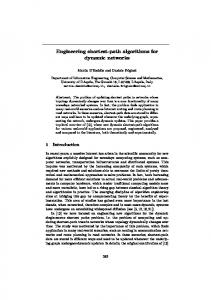
Figure 1: An order graph of four variables. better networks to update the upper bound. At completion, the algorithm finds an optimal network structure that is a subgraph of the initial cyclic graph. If the algorithm ran out of memory before finding the solution, it will switch to using a depth-first search strategy to find a suboptimal solution. Integer linear programming (ILP) has also been used to learn optimal Bayesian network structures (Cussens, 2011; Jaakkola et al., 2010). The learning problem is cast as an integer linear program over a polytope with an exponential number of facets. An outer bound approximation to the polytope is then solved. If the solution of the relaxed problem is integral, it is guaranteed to be the optimal structure. Otherwise, cutting planes and branch and bound algorithms are subsequently applied to find the optimal structure. Recently a similar method has been proposed to find an optimal structure by searching in the space of equivalence classes (Hemmecke et al., 2012). Several other methods can be considered optimal under the constraints that they enforce on the network structure. For example, if optimal parents are selected for each variable, K2 finds an optimal network structure for a particular variable ordering (Cooper & Herskovits, 1992). The methods developed in (Ordyniak & Szeider, 2010; Kojima, Perrier, Imoto, & Miyano, 2010) find an optimal network structure that must be a subgraph of a given super graph.

3. A Shortest Path Perspective This section introduces a shortest path perspective of the problem of learning a Bayesian network structure for a given dataset. 3.1 Order Graph The state space graph for learning Bayesian networks is basically a Hasse diagram containing all of the subsets of the variables in a domain. Figure 1 visualizes the state space graph for a learning problem with four variables. The top-most node with the empty set at layer 29

Yuan & Malone

0 is the start search node, and the bottom-most node with the complete set at layer n is the goal node, where n is the number of variables in a domain. An arc from U to U ∪ {X} represents generating a successor node by adding a new variable {X} to an existing set of variables U; U is called a predecessor of U∪ {X}. The cost of the arc is equal to the score of selecting an optimal parent set for X out of U, i.e., BestScore(X, U). For example, the arc {X1 , X2 } → {X1 , X2 , X3 } has a cost equal to BestScore(X3 , {X1 , X2 }). Each node at layer i has n−i successors as there are this many ways to add a new variable, and i predecessors as there are this many leaf choices. We define expanding a node U as generating all successors nodes of U. With the search graph thus defined, a path from the start node to the goal node is defined as a sequence of nodes such that there is an arc from each of the nodes to the next node in the sequence. Each path also corresponds to an ordering of the variables in the order of their appearance. For example, the path traversing nodes ∅, {X1 }, {X1 , X2 }, {X1 , X2 , X3 }, {X1 , X2 , X3 , X4 } stands for the variable ordering X1 , X2 , X3 , X4 . That is why we also call the search graph an order graph. The cost of a path is defined as the sum of the costs of all the arcs on the path. The shortest path is then the path with the minimum total cost in the order graph. Given the shortest path, we can reconstruct a Bayesian network structure by noting that each arc on the path encodes the choice of optimal parents for one of the variables out of the preceding variables, and the complete path represents an ordering of all the variables. Therefore, putting together all the optimal parent choices generates a valid Bayesian network. By construction, the Bayesian network structure is optimal. 3.2 Finding the Shortest Path Various methods can be applied to solve the shortest path problem. Dynamic programming is considered to evaluate the order graph using a top down sweep of the order graph (Silander & Myllymaki, 2006; Malone et al., 2011b). Layer by layer, dynamic programming finds an optimal subnetwork for the variables contained in each node of the order graph based on results from the previous layers. For example, there are three ways to construct a Bayesian network for node {X1 , X2 , X3 }: using {X2 , X3 } as the subnetwork and X1 as the leaf, using {X1 , X3 } as the subnetwork and X2 as the leaf, or using {X1 , X2 } as the subnetwork and X3 as the leaf. The top-down sweep makes sure that optimal subnetworks are already found for {X2 , X3 }, {X1 , X3 }, and {X1 , X2 }. We only need to select optimal parents for the leaves and identify the leaf that produces the optimal network for {X1 , X2 , X3 }. Once the evaluation reaches the node in the last layer, a shortest path and, equivalently, an optimal Bayesian network are found for the global variable set. A drawback of the dynamic programming approach is its need to compute all the BestScore(.) of all candidate parent sets for each variable. For n variables, there are 2n nodes in the order graph, and there are also 2n−1 parent scores to be computed for each variable, totally n2n−1 scores. As the number of variables increases, computing and storing the order and parent graphs quickly becomes infeasible. In this paper, we propose to apply the A* algorithm (Hart, Nilsson, & Raphael, 1968) to solve the shortest path problem. A* uses the heuristic function to evaluate the quality of search nodes and only expand the most promising search node at each search step. Because 30


of the guidance of the heuristic functions, A* only needs to explore part of the search graph in finding the optimal solution. However, in comparison to dynamic programming, A* has the overhead of calculating heuristic values and maintaining a priority queue. The actual relative performance between dynamic programming and A* thus depends on the efficiency in calculating the heuristic values and the tightness of these values (Felzenszwalb & McAllester, 2007; Klein & Manning, 2003).

4. Finding Optimal Parent Sets Before introducing our algorithm for solving the shortest path problem, we first discuss how to obtain the cost BestScore(X, U) for each arc U → U ∪ {X} that we will visit in the order graph. Recall that each arc involves selecting optimal parents for a variable from a candidate set. We need to consider all subsets of the candidate set in finding the subset with the best score. In this section, we introduce two data structures and related methods for computing and storing optimal parent sets and scores for all pairs of variable and candidate parent set. All exact algorithms for learning Bayesian network structures need to calculate the optimal parent sets and scores. We present a reasonable approach to the calculation in this paper. Note, however, our approach is applicable to other algorithms, and vice versa. 4.1 Parent Graph We use a data structure called parent graph to compute costs for the arcs of the order graph. Each variable has its own parent graph. The parent graph for variable X is a Hasse diagram consisting of all subsets of the variables in V \ {X}. Each node U stores the optimal parent set PAX out of U which minimizes Score(X, PA X ) as well as BestScore(X, U) itself. For example, Figure 2(b) shows a sample parent graph for X1 that contains the best scores of all subsets of {X2 , X3 , X4 }. To obtain Figure 2(b), however, we first need to calculate the preliminary graph in Figure 2(a) that contains the raw score of each subset U as the parent set of X1 , i.e., Score(X1 , U). As Equation 3 shows, these scores can be calculated based on the counts for particular instantiations of the parent and child variables. We use an AD-tree (Moore & Lee, 1998) to collect all the counts from a dataset and compute the scores. An AD-tree is an unbalanced tree structure that contains two types of nodes, AD-tree nodes and varying nodes. An AD-tree node stores the number of data points consistent with a particular variable instantiation; a varying node is used to instantiate the state of a variable. A full AD-tree stores counts of data points that are consistent with all partial instantiations of the variables. A sample AD-tree for two variables are shown in Figure 3. For n variables with d states each, the number of AD-tree nodes in an AD-tree is (d+1)n . It grows even faster than the size of an order or parent graph. Moore and Lee (1998) also described a sparse AD-tree which significantly reduces the space complexity. Readers are referred to that paper for more details. Our pseudo code assumes a sparse AD-tree is used. Given an AD-tree, we are ready to calculate the raw scores Score(X1 , .) for Figure 2(a). There is an exponential number of scores in each parent graph. However, not all parent sets can possibly be in the optimal Bayesian network; certain parent sets can be discarded without ever calculating their values according to the following theorems by Tian (2000). 31

Yuan & Malone

Figure 2: A sample parent graph for variable X1 . (a) The raw scores Score(X1 , .) for all the parent sets. The first line in each node gives the parent set, and the second line gives the score of using all of that set as the parents for X1 . (b) The optimal scores BestScore(X1 , .) for each candidate parent set. The second line in each node gives the optimal score using some subset of the variables in the first line as parents for X1 . (c) The optimal parent sets and their scores. The pruned parent sets are shown in gray. A parent set is pruned if any of its predecessors has a better score.

X1 = * X2 = * C = 50 Vary V X1

Vary V X2

X1 = 0 X2 = *

X1 = 1 X2 = *

X1 = * X2 = 0

X1 = * X2 = 1

C = 20

C = 30

C = 25

C = 25

Vary X2

Vary X2

X1 = 0 X2 = 0

X1 = 0 X2 = 1

X1 = 1 X2 = 0

X1 = 1 X2 = 1

C = 15

C=5

C = 10

C = 20

Figure 3: An AD-tree. We use these theorems to compute only the necessary MDL scores. Other scoring functions such as BDeu also have similar pruning rules (de Campos & Ji, 2011). Algorithm 1 provides the pseudo code for calculating the raw scores. Theorem 1 In an optimal Bayesian network based on the MDL scoring function, each 2N variable has at most ⌊log( log N )⌋ parents, where N is the number of data points. 32


Algorithm 1 Score Calculation Algorithm Input: AD – sparse AD-tree of input data; V – input variables. Output: Score(X, U) for each pair of X ∈ V and U ⊆ V \ {X} 1: function calculateMDLScores(AD, V) 2: for each Xi ∈ V do 3: calculateScores(Xi , AD) 4: end for 5: end function 6: 7: 8: 9: 10: 11: 12: 13: 14: 15: 16: 17: 18: 19: 20: 21: 22: 23: 24: 25: 26: 27:

function calculateScores(Xi, AD) 2N for k ← 0 to ⌊log( log ⊲ Prune due to Theorem 1 N )⌋ do for each U such that U ⊆ V \ {X}& |U| == k do ⊲ All parent sets of size k prune ← f alse for each Y ∈ U do if K(Xi |U) - Score(Xi , U \ {Y }) > 0 then prune ← true ⊲ Prune due to Theorem 2 break end if end for if prune ! = true then Score(Xi , U) ← log2 N K(Xi |U) ⊲ Complexity term for each instantiation xi , u of Xi , U do ⊲ Log likelihood term cF amily ← GetCount({xi } ∪ u,AD) cP arents ← GetCount(u, AD) Score(Xi , U)← Score(Xi , U) - cF amily ∗ log cF amily Score(Xi , U)← Score(Xi , U) + cF amily ∗ log cP arents end for end if end for end for end function

Theorem 2 Let U and S be two candidate parent sets for X, U ⊂ S, and K(Xi |S) − M DL(Xi |U) > 0. Then S and all supersets of S cannot possibly be optimal parent sets for X. After computing the raw scores, we compute the parent graph according to the following theorem which has appeared in many earlier papers, e.g., see the work of Teyssier and Koller (2005), and de Campos and Ji (2010). The theorem simply means that a parent set is not optimal when a subset has a better score. Theorem 3 Let U and S be two candidate parent sets for X such that U ⊂ S, and Score(X, U) ≤ Score(X, S). Then S is not the optimal parent set of X for any candidate set. 33

Yuan & Malone

Algorithm 2 Computing parent graphs Input: All necessary Score(X, U), X ∈ V&U ⊆ V \ {X} Output: Full parent graphs containing BestScore(X, U) 1: function calculateFullParentGraphs(V, Score(., .)) 2: for each X ∈ V do 3: for layer ← 0 to n do ⊲ Propagate best scores down the graph 4: for each U such that U ⊆ V \ {X}& |U| == layer do 5: calculateBestScore(X, U, Score(., .)) 6: end for 7: end for 8: end for 9: end function 10: 11: 12: 13: 14: 15: 16: 17:

function calculateBestScore(X, U, Score(., .)) BestScore(X, U) ← Score(X, U) for each Y ∈ U do if BestScore(X, U \ {Y }) < BestScore(X, U) then BestScore(X, U) ← BestScore(X, U \ {Y }) end if end for end function

function getBestScore(X, U) 19: return BestScore(X, U) 20: end function

⊲ Propagate best scores

⊲ Query BestScore(X, U)

18:

Therefore, when we generate a successor node U∪{Y } of U in the parent graph of X, we check whether Score(X, U ∪ {Y }) is smaller than BestScore(X, U). If so, we let the parent graph node U∪{Y } record itself as the optimal parent set. Otherwise if BestScore(X, U) is smaller, we propagate the optimal parent set in U to U∪{Y }. Because of such propagation, we must have the following (Teyssier & Koller, 2005). Theorem 4 Let U and S be two candidate parent sets for X such that U ⊂ S. We must have BestScore(X, S) ≤ BestScore(X, U). A pseudo code for propagating the scores and computing the parent graph is outlined in Algorithm 2. Figure 2(b) shows the parent graph with the optimal scores after propagating the best scores from top to bottom. During the search of the order graph, whenever we visit a new arc U → U ∪ {X}, we find its score by looking up the parent graph of variable X. For example, if we need to find optimal parents for X1 out of {X2 , X3 }, we look up the node {X2 , X3 } in X1 ’s parent graph to find the optimal parent set and its score. To make the look-ups efficient, we use hash tables to organize the parent graphs so that the query can be answered in constant time. 34


parentsX1 scoresX1

{X2 , X3 } 5

{X3 } 6

{X2 } 8

{} 10

Table 1: Sorted scores and parent sets for X1 after pruning parent sets which are not possibly optimal. parentsX1 2 parentsX X1 X3 parentsX1 4 parentsX X1

{X2 , X3 } 1 1 0

{X3 } 0 1 0

{X2 } 1 0 0

{} 0 0 0

Table 2: The parentsX (Xi ) bit vectors for X1 . A “1” in line Xi indicates that the corresponding parent set includes variable Xi , while a “0” indicates otherwise. Note that, after pruning, none of the optimal parent sets include X4 .

4.2 Sparse Parent Graphs The full parent graph for each variable X exhaustively enumerates all subsets of V \ {X} and stores BestScore(X, U) for all of those subsets. Naively, this approach requires storing n2n−1 scores and parent sets (Silander & Myllymaki, 2006). Because of Theorem 3, however, the number of optimal parent sets is often far smaller than the full size. Figure 2(b) shows that an optimal parent set may be shared by several candidate parent sets. The full parent graph representation will allocate space for this repetitive information for all candidate sets, resulting in waste of time and space. To address these limitations, we introduce a sparse representation of the parent graphs and related scanning techniques for querying optimal parent sets. As with the full parent graphs, we begin by calculating and pruning scores as described in the last Section. Due to Theorems 1 and 2, some of the parent sets can be pruned without being evaluated. Therefore, we do not have to create the full parent graphs. Also, instead of creating the Hasse diagrams, we sort all the optimal parent scores for each variable X in a list, and also maintain a parallel list that stores the associated optimal parent sets. We call these sorted lists scoresX and parentsX . Table 1 shows the sorted lists for the optimal scores in the parent graph in Figure 2(b). In essence, this allows us to store and efficiently process only the scores in Figure 2(c). To find the optimal parent set for X out of a candidate set U, we can simply scan the list of X starting from the beginning. As soon as we find the first parent set that is a subset of U, we find the optimal parent score BestScore(X, U). This is trivially true due to the following theorem. Theorem 5 The first subset of U in parentsX is the optimal parent set for X out of U. Scanning the lists to find optimal parent sets can be inefficient if not done properly. Since we have to do the scanning for each arc visited in the order graph, any inefficiency in the scanning can have a large impact on the search algorithm. 35

Yuan & Malone

parentsX1 validX1 3 ∼ parentsX X1 new validX1

{X2 , X3 } 1 0 0

{X3 } 1 0 0

{X2 } 1 1 1

{} 1 1 1

Table 3: The result of performing the bitwise operation to exclude all parent sets which include X3 . A “1” in the validX1 bit vector means that the parent set does not include X3 and can be used for selecting the optimal parents. The first set bit indicates the best possible score and parent set.

parentsX1 validX1 3 ∼ parentsX X1 new validX1

{X2 , X3 } 0 0 0

{X3 } 0 1 0

{X2 } 1 0 0

{} 1 1 1

Table 4: The result of performing the bitwise operation to exclude all parent sets which include either X3 or X2 . A “1” in the validnew X1 bit vector means that the parent set includes neither X2 nor X3 . The initial validX1 bit vector had already excluded X3 , so finding validnew X1 only required excluding X2 .

To ensure the efficiency, we propose the following scanning technique. For each variable X, we first initialize a working bit vector of length kscoresX k called validX to be all 1s. This indicates that all the parent scores in scoresX are usable. Then, we create n − 1 bit vectors also of length kscoresX k, one for each variable in V \ {X}. The bit vector for variable Y is denoted as parentsYX and contains 1s for all the parent sets that contain Y and 0s for others. Table 2 shows the bit vectors for the example in Table 1. Then, to exclude variable Y as a candidate parent, we perform the bit operation validnew ← validX & ∼ parentsYX . The new X validX bit vector now contains 1s for all the parent sets that are subsets of V \ {Y }. The first set bit corresponds to BestScore(X, V \ {Y }). Table 3 shows an example of excluding X3 from the set of possible parents for X1 , and the first set bit in the new bit vector corresponds to BestScore(X1 , V \ {X3 }). If we further want to exclude X2 as a candidate parent, the new bit vector from the last step becomes the current bit vector for this step, 2 and the same bit operation is applied: validnew ← validX & ∼ parentsX X X1 . The first set bit of the result corresponds to BestScore(X1 , V \ {X2 , X3 }). Table 4 demonstrates this operation. Also, it is important to note that we exclude one variable at a time. For example, if, after excluding X3 , we wanted to exclude X4 rather than X2 , we could take validnew ← X 4 validX & ∼ parentsX . These operations are described in the createSparseParentGraph and X getBestScore functions in Algorithm 3. Because of the pruning of duplicate scores, the sparse representation requires much less memory than storing all the possible parent sets and scores. As long as kscores(X)k < C(n − 1, n2 ), it also requires less memory than the memory-efficient dynamic programming algorithm (Malone et al., 2011b). Experimentally, we show that kscoresX k is almost 36


Algorithm 3 Sparse Parent Graph Algorithms Input: All necessary Score(X, U), X ∈ V&U ⊆ V \ {X} Output: Sparse parent graphs containing optimal parent sets and scores 1: function createSparseParentGraph(X, Score(., .)) 2: for X ∈ V do 3: scorest , parentst ←sort(Score(X, ·)) ⊲ Sort scores, preferring low cardinality 4: scoresX , parentsX ← ∅ ⊲ Initialize possibly optimal scores 5: for i = 0 → |scorest | do 6: prune ← f alse 7: for j = 0 → |scoresX | do ⊲ Check if a better subset pattern exists 8: if contains(parentst(i), parentsX (j))&scoresX (i) ≤ scorest (i) then 9: prune ← true 10: Break 11: end if 12: end for 13: if prune ! = true then 14: Append scoresX , parentsX with parentst(i), parentst (i) 15: end if 16: end for 17: for i = 0 → |scoresX | do ⊲ Set bit vectors for efficient querying 18: for each Y ∈ parentsX (i) do 19: set(parentsYX (i)) 20: end for 21: end for 22: end for 23: end function 24: 25: 26: 27: 28: 29: 30: 31:

function getBestScore(X, U) valid ← allScoresX for each Y ∈ V \ U do valid ← valid& ∼ parentsYX end for f sb ← f irstSetBit(valid) return scoresX [f sb] end function

⊲ Query BestScore(X, U)

⊲ Return the first score with a set bit

always smaller than C(n − 1, n2 ) by several orders of magnitude. So this approach offers (usually substantial) memory savings compared to previous best approaches. The sparse representation has an extra benefit of improving the time efficiency as well. With the full representation, we have to create the complete exponential-size parent graphs, even though many nodes in a parent graph share the same optimal parent choices. With the sparse representation, we can avoid creating those nodes, which makes creating the sparse parent graphs much more efficient. 37

Yuan & Malone

5. An A* Search Algorithm We are now ready to tackle the shortest path problem in the order graph. This section presents our search algorithm as well as two admissible heuristic functions for guiding the algorithm. 5.1 The Algorithm We apply a well known state space search method, the A* algorithm (Hart et al., 1968), to solve the shortest path problem in the order graph. The main idea of the algorithm is to use an evaluation function f to measure the quality of search nodes and always expand the one that has the lowest f cost during the exploration of the order graph. For a node U, f (U) is decomposed as the sum of an exact past cost, g(U), and the estimated future cost, h(U). The g(U) cost measures the shortest distance from the start node to U, while the h(U) cost estimates how far away U is from the goal node. Therefore, the f cost provides an estimated total cost of the best possible path which passes through U. A* uses an open list (usually as a priority queue) to store the search frontier, and a closed list to store the expanded nodes. Initially the open list only contains the start node, and the closed list is empty. At each search step, the node with the lowest f -cost from the open list, say U, is selected for expansion to generate its successor nodes. Before expanding U, however, we need to first check whether it is the goal node. If yes, a shortest path to the goal has been found; we can construct a Bayesian network from the path and terminate the search. If U is not the goal, we expand it to generate the successor nodes. Each successor S considers one possible way of adding a new variable, say X, as a leaf to an existing subnetwork over the variables in U, that is S = U ∪ {X}. The g cost of S is calculated as the sum of the g-cost of U and the cost of the arc U → S. The arc cost as well as the optimal parent set PAX for X out of U are retrieved from X’s parent graph. The h cost of S is computed from a heuristic function which we will describe shortly. We record in S the following information2 : g cost, h cost, X, and PAX . It is clear from the order graph that there are multiple paths to any node. We should perform duplicate detection for S to see whether a node representing the same set of variables has already been generated before. If we do not check for duplicates, the search space blows up from an order graph with a size 2n to an order tree with a size n!. We first check whether a duplicate already exists in the closed list. If so, we further check whether the duplicate has a better g cost than S. If yes, we discard S immediately, as it represents a worse path. Otherwise, we remove the duplicate from the closed list, and place S in the open list. What happens is we have found a better path with a lower g cost, so we reopen the node for future search. If no duplicate is found in the closed list, we also need to check the open list. If no duplicate is found, we will simply add S to the open list. Otherwise, we will compare the g costs of the duplicate and S. If the duplicate has a lower g cost, S will be discarded. Otherwise, we will replace the duplicate with S. Again, the lower g cost means a better path is found. 2. We can also delay the calculation of h until after duplicate detection to avoid unnecessary calculations for nodes that will be pruned.

38


Algorithm 4 A* Search Algorithm Input: full or sparse parent graphs containing BestScore(X, U) Output: an optimal Bayesian network G 1: function main(D) 2: start ← ∅ 3: Score(start) ← 0 P 4: push(open, start, Y ∈V BestScore(Y, V \ {Y }) 5: while !isEmpty(open) do 6: U ←pop(open) 7: if U is goal then ⊲ A shortest path is found 8: print(“The best score is ” + Score(V)) 9: G ← construct a network from the shortest path 10: return G 11: end if 12: put(closed, U) 13: for each X ∈ V \ U do ⊲ Generate successors 14: g ← BestScore(X, U) + Score(U) 15: if contains(closed, U ∪ {X}) then ⊲ Closed list DD 16: if g < Score(U ∪ {X}) then ⊲ reopen node 17: delete(closed, U ∪ {X}) 18: push (open, U ∪ {X}, g + h) 19: Score(U ∪ {X}) ← g 20: end if 21: else 22: if contains(open, U ∪ {X}) & g < Score(U ∪ {X}) then⊲ Open list DD 23: update(open, U ∪ {X}, g + h) 24: Score(U ∪ {X}) ← g 25: end if 26: end if 27: end for 28: end while 29: end function

After all the successor nodes have been generated, we will place node U in the closed list, which indicates that node is already expanded. Expanding the top node in the open list is called one search step. The A* algorithm performs the step repeatedly until the goal node is selected for expansion. At that moment a shortest path from the start state to the goal state has been found. Once the shortest path is found, we can reconstruct the optimal Bayesian network structure by starting from the goal node and tracing back the shortest path until reaching the start node. Since each node on the path stores a leaf variable and its optimal parent set, putting all the optimal parent sets together generates a valid Bayesian network structure. A pseudo code of the A* algorithm is shown in Algorithm 4. 39

Yuan & Malone

5.2 A Simple Heuristic Function The A* algorithm provides different theoretical guarantees depending on the properties of the heuristic function h. The function h is admissible if the h cost is never greater than the true cost to the goal; in other words, it is optimistic. Given an admissible heuristic function, the A* algorithm is guaranteed to find the shortest path once the goal node is selected for expansion (Pearl, 1984). Let U be a node in the order graph. We first consider the following simple heuristic function h. Definition 1 h(U) =

X

BestScore(X, V\{X}).

(7)

X∈V\U

The heuristic function allows each remaining variable to choose optimal parents from all the other variables. Its design reflects the principle that the exact cost of a relaxed problem can be used as an admissible bound for the original problem (Pearl, 1984). In this case, the original problem is to learn a Bayesian network that is a directed acyclic graph. Equation 7 relaxes the problem by ignoring the acyclicity constraint, so all directed cyclic graphs are allowed. The heuristic function is easily proven admissible in the following theorem. The proofs of all the theorems in this paper can be found in Appendix A. Theorem 6 h is admissible. It turns out that h has an even nicer property. A heuristic function is consistent if, for any node U and a successor S, h(U) ≤ h(S) + c(U, S), where c(U, S) stands for the cost of the arc U → S. Given a consistent heuristic, the f cost is monotonically non-decreasing following any path in the order graph. As a result, the f cost of any node is less than or equal to the f cost of the goal node. It follows immediately that a consistent heuristic is guaranteed to be admissible. With a consistent heuristic, the A* algorithm is guaranteed to find the shortest path to any node U once U is selected for expansion. If a duplicate is found in the closed list, the duplicate must have the optimal g cost, so the new node can be discarded immediately. We show in the following that the simple heuristic in Equation 7 is also consistent. Theorem 7 h is consistent. The heuristic may seem expensive to compute as it requires computing BestScore(X, V\ {X}) for each variable X. However, these scores can be easily found by querying the parent graphs and are stored in an array for repeated use. It takes linear time to calculate the heuristic for the start node. Any subsequent computation of h, however, only takes constant time because we can simply subtract the best score of the newly added variable from the heuristic value of the parent node. 5.3 An Improved Admissible Heuristic The simple heuristic function defined in Equation 7, referred to as hsimple hereafter, relaxes the acyclicity constraint of Bayesian networks completely. As a result, hsimple may introduce many directed cycles and result in a loose bound. We introduce another heuristic in this section to tighten the heuristic. We first use a toy example to motivate the new heuristic, and then describe two specific approaches to computing the heuristic. 40


X1

X2

X3

X4

Figure 4: A directed graph representing the heuristic estimate for the start search node.

5.3.1 A Motivating Example With hsimple , the heuristic estimate of the start node in an order graph allows each variable to choose optimal parents from all the other variables. Suppose the optimal parent sets for X1 , X2 , X3 , X4 are {X2 , X3 , X4 }, {X1 , X4 }, {X2 }, {X2 , X3 } respectively. These parent choices are shown as the directed graph in Figure 4. Since the acyclicity constraint is ignored, directed cycles are introduced, e.g., between X1 and X2 . However, we know the final solution cannot have cycles; three cases are possible between X1 and X2 : (1) X2 is a parent of X1 (so X1 cannot be a parent of X2 ), (2) X1 is a parent of X2 , or (3) neither of the above is true. Based on Theorem 4, the third case cannot provide a better value than the first two cases because one of the variables must have fewer candidate parents. Between (1) and (2), it is unclear which one is better, so we take the minimum of them to get a lower bound. Consider case (1). We have to delete the arc X1 → X2 to rule out X1 as a parent of X2 . Then we have to let X2 rechoose optimal parents from the remaining variables {X3 , X4 }, that is, we must check all parent sets not including X1 . The deletion of the arc alone cannot produce the new bound because the best parent set for X2 out of {X3 , X4 } is not necessarily {X4 }. The total bound of X1 and X2 is computed by summing together the original bound of X1 and the new bound of X2 . We call this total bound b1 . Case (2) is handled similarly; we call that total bound b2 . Because the joint cost for X1 and X2 , c(X1 , X2 ), must be optimistic, we compute it as the minimum of b1 and b2 . Effectively we have considered all possible ways to break the cycle and obtained a tighter heuristic value. The new heuristic is clearly admissible, as we still allow cycles among other variables. Often, hsimple introduces multiple cycles into a heuristic estimate. Figure 4 also has a cycle between X2 and X4 . This cycle shares X2 with the earlier cycle between X1 and X2 ; we say the cycles overlap. One way to break both cycles is to set the parent set of X2 to be {X3 }; however, it introduces a new cycle between X2 and X3 . As described in more detail shortly, we partition the variables into exclusive groups and only break cycles within each group. In this example, if X2 and X3 are in different groups, we do not break the cycle. 41

Yuan & Malone

5.3.2 The K-Cycle Conflict Heuristic The above idea can be generalized to compute the joint cost for any variable group with size up to k by avoiding cycles within the group. Then for any node U in the order graph, we calculate its heuristic value by partitioning the variables V \ U into several exclusive groups and sum their costs together. We name the resulting technique the k-cycle conflict heuristic. Note that the simple heuristic hsimple is a special case of this new heuristic, as it simply contains costs for the individual variables (k=1). The new heuristic is an application of the additive pattern database technique (Felner, Korf, & Hanan, 2004). Pattern databases (Culberson & Schaeffer, 1998) is an approach to computing an admissible heuristic for a problem by solving a relaxed problem. Consider the 15-puzzle problem. 15 square tiles numbered from 1 to 15 are randomly placed in a 4 by 4 box with one position left empty. Each such configuration of the tiles is called a state. The goal is to slide the tiles one at a time into a destination configuration. A tile can slide into the empty position only if it is beside that position. The 15 puzzle can be relaxed to only contain the tiles 1-8 with the other tiles removed. Because of the relaxation, multiple states of the original problem map to one state in the abstract state space of the relaxed problem as they share the positions of the remaining tiles. Each abstract state is called a pattern; the cost of the pattern is equal to the smallest cost for sliding the remaining tiles into their destination positions. The cost provides a lower bound for any state in the original state space which maps to that pattern. The costs of all patterns are stored in a pattern database. We can relax a problem in different ways and obtain multiple pattern databases. If the solutions to several relaxed problems are independent, the problems are said to be exclusive. For the 15-puzzle, we can also relax it to only contain tiles 9-15. This relaxation can be solved independently from the previous one because they do not share any puzzle movements. For any concrete state in the original state space, the positions of tiles 1-8 map it to a pattern in the first pattern database, and the positions of tiles 9-15 map it to a different pattern in the second pattern database. The costs of these patterns can be added together to obtain an admissible heuristic, hence the name additive pattern databases. For our learning problem, a pattern is defined as a group of variables, and its cost is the optimal joint cost of these variables while avoiding directed cycles between them. The decomposability of the scoring function implies that the costs of two exclusive patterns can be added together to obtain an admissible heuristic. We do not have to explicitly break cycles in computing the cost of a pattern. The following theorem offers a straightforward approach to doing so. Theorem 8 The cost of the pattern U, c(U), is equal to the shortest distance from V \ U to the goal node in the order graph. Again consider the example in Figure 4. The cost of pattern {X1 , X2 } is equal to the shortest distance between {X3 , X4 } and the goal in the order graph in Figure 1. Furthermore, the difference between c(U) and the sum of the simple heuristic values of all variables in U indicates the amount of improvement brought by avoiding cycles within the pattern. The differential score, called δh , can thus be used as a quality measure for ordering the patterns and for choosing patterns that are more likely to result in a tighter heuristic. 42


5.3.3 Dynamic K-Cycle Conflict Heuristic There are two slightly different versions of the k-cycle conflict heuristic. In the first version named dynamic k-cycle conflict heuristic, we compute the costs for all groups of variables with size up to k and store them in a single pattern database. According to Theorem 8, this heuristic can be computed by finding the shortest distances between all the nodes in the last k layers of the order graph and the goal. We compute the heuristic by using a breadth-first search to do a backward search in the order graph for k layers. The search starts from the goal node and expands the order graph backward layer by layer. A reverse arc U ∪ {X} → U has the same cost as the arc U → U ∪ {X}, i.e., BestScore(X, U). The reverse g cost of U is updated whenever a new path with a lower cost is found. Breadth-first search ensures that node U will obtain its exact reverse g cost once the previous layer is expanded. The g cost is the cost of the pattern V \ U. We also compute the differential score, δh , for each pattern at the same time. A pattern which does not have a better differential score than any of its subset patterns will be discarded. The pruning can significantly reduce the size of a pattern database and improve its query efficiency. The algorithm for computing the dynamic k-cycle conflict heuristic is shown in Algorithm 5. Once the heuristic is created, we can calculate the heuristic value for each search node as follows. For node U, we partition the remaining variables V \ U into a set of exclusive patterns, and sum their costs together as the heuristic value. Since we only prune superset patterns, we can always find such a partition. However, there are potentially many ways of partition. Ideally we want to find the one with the highest total cost, which represents the tightest heuristic value. The problem of finding the optimal partition can be formulated as maximum weighted matching problem (Felner et al., 2004). For k = 2, we can define an undirected graph in which each vertex represents a variable, and each edge between two variables represents the pattern containing the same variables and has a weight equal to the cost of the pattern. The goal is to select a set of edges from the graph so that no two edges share a vertex and the total weight of the edges is maximized. The matching problem can be solved in O(n3 ) time, where n is the number of vertices (Papadimitriou & Steiglitz, 1982). For k > 2, we have to add hyperedges to the matching graph for connecting up to k vertices to represent larger patterns. The goal becomes to select a set of edges and hyperedges to maximize the total weight. However, the three-dimensional or higher-order maximum weighted matching problem is NP-hard (Garey & Johnson, 1979). That means we have to solve an NP-hard problem when calculating each heuristic value. To alleviate the potential inefficiency, we greedily select patterns based on their quality. Consider node U with unsearched variables V \ U. We choose the pattern with the highest differential cost from all the patterns that are subsets of V \ U. We repeat this step for the remaining variables until all the variables are covered. The total cost of the chosen patterns is used as the heuristic value for U. The hdynamic function of Algorithm 5 gives pseudocode for computing the heuristic value. The dynamic k-cycle conflict heuristic introduced above is an example of the dynamically partitioned pattern database (Felner et al., 2004) because the patterns are dynamically selected during the search algorithm. We refer to it as dynamic pattern database for short. 43

Yuan & Malone

Algorithm 5 Dynamic k-cycle Conflict Heuristic Input: full or sparse parent graphs containing all BestScore(X, U) Output: A pattern database P D with patterns up to size k 1: function createDynamicPD(k) 2: P D0 (V) ← 0 3: δh (V) ← 0 4: for l = 1 → k do ⊲ Perform BFS for k levels 5: for each U ∈ P Dl−1 do 6: expand(U, l) 7: checkSave(U) 8: P D(V \ U) ← P Dl−1 (U) 9: end for 10: end for 11: for each X ∈ P D \ save do ⊲ Remove superset patterns with no improvement 12: delete P D(X) 13: end for 14: sort(P D : δh ) ⊲ Sort patterns in decreasing costs 15: end function 16: 17: 18: 19: 20: 21: 22: 23: 24: 25: 26: 27: 28: 29: 30: 31: 32: 33: 34: 35: 36: 37: 38:

function expand(U, l) for each X ∈ U do g ← P Dl−1 (U) + BestScore(X, U \ {X}) if g < P Dl (U \ {X}) then P Dl (U \ {X}) ← g end for end function

⊲ Duplicate detection

function checkSave(U) P δh (U) ← g − Y ∈V\U BestScore(Y, V \ {Y }) for each X ∈ V \ U do ⊲ Check improvement over subset patterns if δh (U) > δh (U ∪ {X}) then save(U) end for end function function hdynamic (U) h←0 R←U for each S ∈ P D do if S ⊂ R then R←R\S h ← h + P D(S) end if end for return h end function

⊲ Calculate heuristic value for U

⊲ Greedily find best subset pattern of R

44


A potential drawback of dynamic pattern databases is that, even with the greedy method, computing a heuristic value is still much more expensive than the simple heuristic in Equation 7. Consequently, the search time can be longer even though the tighter pattern database heuristic results in more pruning and fewer expanded nodes. 5.3.4 Static K-Cycle Conflict Heuristic To address the inefficiency of dynamic pattern database in computing heuristic values, we introduce another version named static k-cycle conflict heuristic based on the statically partitioned pattern database technique (Felner et al., 2004). The idea is to partition the variables into several static exclusive groups, and create a separate pattern database for each group. Consider a problem with variables {X1 , ..., X8 }. We divide the variables into two groups, {X1 , ..., X4 } and {X5 , ..., X8 }. For each group, say {X1 , ..., X4 }, we create a pattern database that contains the costs of all subsets of {X1 , ..., X4 } and store them as a hash table. We refer to this heuristic as the static pattern database for short.S We create static pattern databases as follows. For a static grouping V = i Vi , we need to compute a pattern database for each group Vi that resembles an order graph containing all subsets of Vi . We use a breadth first search to create the graph starting S from the node Vi . The cost for an arc U∪{X} → U in this graph is equal to BestScore(X, ( j6=i Vj )∪U), which means that the variables in the other groups are valid candidate parents. To ensure efficient retrieval, these static pattern databases are stored as hashtables; nothing is pruned from them. Algorithm 6 gives pseudocode for creating static pattern databases. It is much simpler to use static pattern databases to compute a heuristic value. Consider the search node {X1 , X4 , X8 }; the unsearched variables are {X2 , X3 , X5 , X6 , X7 }. We simply divide these variables into two patterns {X2 , X3 } and {X5 , X6 , X7 } according to the static grouping, look them up in the respective pattern databases, and sum the costs together as the heuristic value. Moreover, since each search step just processes one variable, only one pattern is affected and requires a new score lookup. Therefore, the heuristic value can be calculated incrementally. The hstatic function of Algorithm 6 provides pseudocode for naively calculating this heuristic value. 5.3.5 Properties of The K-Cycle Conflict Heuristic Both versions of the k-cycle conflict heuristic remain admissible. Although they can avoid cycles within each pattern, they cannot prevent cycles across different patterns. The following theorem proves the result. Theorem 9 The k-cycle conflict heuristic is admissible. Understanding the consistency of the new heuristic is slightly more complex. We first look at the static pattern database as it does not involve selecting patterns dynamically. The following theorem shows that the static pattern database is still consistent. Theorem 10 The static pattern database version of the k-cycle conflict heuristic remains consistent. In the dynamic pattern database, each search step needs to solve a maximum weighted matching problem and select a set of patterns to compute the heuristic value. In the 45

Yuan & Malone

Algorithm 6 Static k-cycle Conflict Heuristics S Input: full or sparse parent graphs containing BestScore(X, U), i Vi – a partition of V Output: A full pattern database P D i for each Vi 1: function createStaticPD(Vi ) 2: P D0i (∅) ← 0 3: for l = 1 → Vi do ⊲ Perform BFS over Vi i 4: for each U ∈ P Dl−1 do 5: expand(U, l, Vi ) i (U) 6: P D i (U) ← P Dl−1 7: end for 8: end for 9: end function 10: 11: 12: 13: 14: 15: 16: 17: 18: 19: 20: 21: 22:

function expand(U, l, Vi ) for each X ∈ Vi \ U do S i (U) + BestScore(X, U g ← P Dl−1 j6=i Vj ) i i if g < P Dl (U ∪ X) then P Dl (U ∪ X) ← g end for end function function hstatic (U) h←0 for each Vi ⊂ V do h ← h + P D i (U ∩ Vi ) end for return h end function

⊲ Duplicate detection

⊲ Sum over each P D i separately

following, we show that the dynamic k-cycle conflict heuristic is also consistent by closely following that of Theorem 4.1 in the work of Edelkamp and Schrodl (2012). Theorem 11 The dynamic pattern database version of the k-cycle conflict heuristic remains consistent. However, the above theorem assumes the use of the shortest distances between the nodes in the abstract space. Because we use a greedy method to solve the maximum weighted matching problem, we can no longer guarantee to find the shortest paths. As a result, we may lose the consistency property of the dynamic pattern database. It is thus necessary for A* to reopen a duplicate node in the closed list if a better path is found.

6. Experiments We evaluated the A* search algorithm on a set of benchmark datasets from the UCI repository (Bache & Lichman, 2013). The datasets have up to 29 variables and 30, 162 data points. We discretized all variables into two states using the mean values and deleted all 46


1.00E+10 1.00E+09

Full

Largest Layer

Sparse

1.00E+08 1.00E+07

Size

1.00E+06 1.00E+05 1.00E+04 1.00E+03 1.00E+02 1.00E+01 1.00E+00

Figure 5: The number of parent sets and their scores stored in the full parent graphs (“Full”), the largest layer of the parent graphs in memory-efficient dynamic programming (“Largest Layer”), and the sparse representation (“Sparse”).

the data points with missing values. Our A* search algorithm is implemented in Java3 . We compared our algorithm against the branch and bound (BB)4 (de Campos & Ji, 2011), dynamic programming (DP)5 (Silander & Myllymaki, 2006), and integer linear programming (GOBNILP) algorithms6 (Cussens, 2011). We used the latest versions of these software or source code at the time of the experiments as well as their default parameter settings; it was version 1.1 for GOBNILP and 2.1.1 for SCIP. BB and DP do not calculate MDL, but they use the BIC score, which uses an equivalent calculation as MDL. Our results confirmed that the algorithms found Bayesian networks that either are the same or belong to the same equivalence class. The experiments were performed on a 2.66 GHz Intel Xeon with 16GB of RAM and running SUSE Linux Enterprise Server version 10. 6.1 Full vs Sparse Parent Graphs We first evaluated the memory savings made possible by the sparse parent graphs in comparison to the full parent graphs. In particular, we compared the maximum number of scores that have to be stored for all variables at once by each algorithm. A typical dynamic programming algorithm stores scores for all possible parent sets of all variables. The memory-efficient dynamic programming (Malone et al., 2011b) stores all possible parent sets only in one layer of the parent graphs for all variables, so the size of the largest layer of 3. A software package with source code named URLearning (“You Are Learning”) implementing the A* algorithm can be downloaded at http://url.cs.qc.cuny.edu/software/URLearning.html. 4. http://www.ecse.rpi.edu/∼cvrl/structlearning.html 5. http://b-course.hiit.fi/bene 6. http://www.cs.york.ac.uk/aig/sw/gobnilp/

47

Yuan & Malone

all parent graphs is an indication of its space requirement. The sparse representation only stores the optimal parent sets for all variables. Figure 5 shows the memory savings by the sparse representation on the benchmark datasets. It is clear that the number of optimal parent scores stored by the sparse representation is typically several orders of magnitude smaller than the full representation. Furthermore, due to Theorem 1, increasing the number of data points increases the maximum number of candidate parents. Therefore, the number of candidate parent sets increases as the number of data points increases; however, many of the new parent sets are pruned in the sparse representation because of Theorem 3. The number of variables also affects the number of candidate parent sets. Consequently, the number of optimal parent scores increases as a function of the number of data points and the number of variables. As the results show, the amount of pruning is data-dependent, though, and not easily predictable. In practice, we find the number of data points to affect the number of unique scores much more than the number of variables. 6.2 Pattern Database Heuristics The new pattern database heuristic has two versions: static and dynamic pattern databases; each of them can be parameterized in different ways. We tested various parameterizations of the new heuristics on the A* algorithm on two datasets named Autos and Flag. We chose these two datasets because they have a large enough number of variables and can better demonstrate the effect of pattern database heuristics. For the dynamic pattern database, we varied k from 2 to 4. For the static pattern databases, we tried groupings 9-9-8 and 13-13 for the Autos dataset and groupings 10-10-9 and 15-14 for the Flag dataset. We obtained the groupings by simply dividing the variables in the datasets into several consecutive blocks. The results based on the sparse parent graphs are shown in Figure 6. We did not show the results of full parent graphs because A* ran out of memory on both datasets when full parent graphs were used. With the sparse representations, A* achieved much better scalability, and was able to solve both Autos with any heuristic and Flag with some of the best heuristics when using sparse parent graphs. Hereafter our experiments and results assume the use of sparse parent graphs. Also, the pattern database heuristics improved the efficiency and scalability of A* significantly. A* with either the simple heuristic or the static pattern database with grouping 10-10-9 ran out of memory on the Flag dataset. The other pattern database heuristics enabled A* to finish successfully. The dynamic pattern database with k = 2 helped to reduce the number of expanded nodes significantly on both datasets. Setting k = 3 helped even more. However, further increasing k to 4 resulted in increased search time, and sometimes even an increased number of expanded nodes (not shown). We believe that a larger k always results in a better pattern database; the occasional increase in expanded nodes is because the greedy strategy we used to choose patterns did not fully utilize the better heuristic. The longer search time is more understandable though, because it is less efficient to compute a heuristic value in larger pattern databases, and the inefficiency gradually overtook the benefit. Therefore, k = 3 seems to be the best parametrization for the dynamic pattern database in general. For the static pattern databases, we were able to test much larger 48


1.00E+04

Running Time

Size of Pattern Database

1.00E+05

1.00E+03 1.00E+02 1.00E+01 1.00E+00

500 450 400 350 300 250 200 150 100 50 0

Autos

1.00E+04

Running Time

Size of Pattern Database

1.00E+05

1.00E+03 1.00E+02 1.00E+01 1.00E+00

500 450 400 350 300 250 200 150 100 50 0

X

X

F lag Figure 6: A comparison of A* enhanced with different heuristics (hsimple , hdynamic with k = 2, 3, and 4, and hstatic with groupings 9-9-8 and 13-13 for the Autos dataset and groupings 10-10-9 and 15-14 for the Flag dataset). “Size of Pattern Database” means the number of patterns stored. “Running Time” means the search time (in seconds) using the indicated pattern database strategy. An “X” means out of memory.

groups because we do not need to enumerate all groups up to a certain size. The results suggest that fewer larger groups tend to result in tighter heuristic. The sizes of the static pattern databases are typically much larger than the dynamic pattern databases. However, the time needed to create the pattern databases is still negligible in comparison to the search time in all cases. It is thus cost effective to try to compute larger but affordable-size static pattern databases to achieve better search efficiency. Our results show that the best static pattern databases typically helped A* to achieve better efficiency than the dynamic pattern databases, even when the number of expanded nodes is larger. The reason is that calculating the heuristic values is much more efficient when using static pattern databases. 49

Yuan & Malone

10000 BB Scoring

DP Scoring

A* Scoring

Scoring Time

1000

100

10

1

0.1

Figure 7: A comparison of the scoring time of the BB, DP, and A* algorithms. Each label of the X-axis consists of a dataset name, the number of variables, and the number of data points.

6.3 A* with the Simple Heuristic We first tested A* with the hsimple heuristic. Each competing algorithm has roughly two phases, computing optimal parent sets/scores (scoring phase) and searching for a Bayesian network structure (searching phase). We therefore compare the algorithms based on two parts of running time: scoring time and search time. Figure 7 shows the scoring times of BB, DP, and A*. GOBNILP was not included because it assumes the optimal scores are provided as input. Each label in the horizontal axis shows a dataset, the number of variables, and the number of data points. The results show that the AD-tree method used in our A* algorithm seems to be the most efficient approach to computing the parent scores. The scoring part of DP is often more than an order of magnitude slower than others. This result is somewhat misleading, however. The scoring and searching parts of DP are more tightly integrated than the other algorithms. As a result, most of the work in DP is done in the scoring part; little work is left for the search. As we will show shortly, the search time of DP is typically very short. Figure 8(a) reports the search time of all the algorithms. Some of the benchmark datasets are so difficult that some algorithms take too long or even fail to find the optimal solutions. We therefore terminate an algorithm early if it runs for more than 7,200 seconds on a dataset. The results show that BB only succeeded on two of the datasets, Voting and Hepatitis, within the time limit. On both datasets, the A* algorithm is several orders of magnitude faster than BB. The major difference between A* and BB is the formulation of the search space. BB searches in the space of directed cyclic graphs, while A* always maintains a directed acyclic graph during the search. The results indicate that it is better to search in the space of directed acyclic graphs. The results also show that the search time needed by the DP algorithm is often shorter than A*. As we explained earlier, the reason is that all the heavy lifting in DP is done in 50


10000 BB

DP

GOBNILP

A*

Search Time

1000

100

10

1

X X

X

X

X

X

X

X

X X

X

(a) 10000

Total Running Time

DP Total Time

A* Total Time

1000

100

10

1

(b) Figure 8: A comparison of the (a) search time (in seconds) for BB, DP, GOBNILP, and A* and (b) total running time for DP and A*. An “X” means that the corresponding algorithm did not finish within the time limit (7,200 seconds) or ran out of memory in the case of A*. . the scoring part. If we add the scoring and search time together, as shown in Figure 8(b), A* is several times faster than DP on all the datasets except Adult and Voting (Again, GOBNILP is left out because it only has the search part). The main difference between A* and DP is that A* only explores part of the order graph, while dynamic programming fully evaluates the graph. However, each step of the A* search algorithm has some overhead cost for computing the heuristic function and maintaining a priority queue. One step 51

Yuan & Malone

of A* is more expensive than a similar dynamic programming step. If the pruning does not outweigh its overhead, A* can be slower than dynamic programming. Both Adult and Voting have a large number of data points, which makes the pruning technique in Theorem 1 less effective. Although the DP algorithm does not perform any pruning, due to its simplicity, the algorithm can be highly streamlined and optimized in performing all its calculations. That is why the DP algorithm was faster than A* search on these two datasets. However, our A* algorithm was more efficient than DP on all the other datasets. For these datasets, the number of data points is not that large in comparison to the number of variables. The pruning significantly outweighs the overhead of A*. As an example, A* runs faster on the Mushroom dataset when comparing total running time even though Mushroom has over 8,000 data points. The comparison between GOBNILP and A* shows that they each has its own advantages. A* was able to find optimal Bayesian networks for all the datasets well within the time limit. GOBNILP failed to learn optimal Bayesian networks for three of the datasets, including Letter, Image, and Mushroom. The reason is that GOBNILP formulates the learning problem as an integer linear program whose variables correspond to the optimal parent sets of all variables. Even though these datasets do not have many variables, they have many optimal parent sets, so the integer programs for them have too many variables to be solvable within the time limit. On the other hand, the results also show that GOBNILP was quite efficient on many of the other datasets. Even though a dataset may have many variables, GOBNILP can solve it efficiently as long as the number of optimal parent sets is small. It is much more efficient than A* on datasets such as Hepatitis and Heart, although the opposite is true on datasets such as Adult and Statlog. 6.4 A* with Pattern Database Heuristics Since static pattern databases seem to work better than dynamic pattern databases in most cases, we tested A* with static pattern database (A*,SP) against A*, DP, and GOBNILP on all the datasets used in Figure 8 as well as several larger datasets. We used the simple static grouping of ⌈ n2 ⌉ − ⌊ n2 ⌋ for all the datasets, where n is the number of variables. The results of BB are excluded because it did not solve any additional dataset. The results are shown in Figure 9. The benefits brought by the pattern databases for A* are rather obvious. For the datasets on which A* was able to finish, A*,SP was typically up to an order of magnitude faster. In addition, A*,SP was able to solve three larger datasets: Sensor, Autos, and Flag, while A* failed on all of them. The running time on each of those datasets is pretty short, which indicates that once the memory consumption of the parent graphs was reduced, A* was able to use more memory for the order graph and solve the search problems rather easily. DP was able to solve one more dataset, Autos, which A* was not able to solve. It is somewhat surprising given that A* has pruning capability. The explanation is that A* stores all search information in RAM, so it will fail once the RAM is exhausted. The DP algorithm described by Silander and Myllymaki (2006) stores its intermediate results as computer files on hard disks, so it was able to scale to larger datasets than A*. 52


1000

Search Time

DP

GOBNILP

A*

A*, SP

100

10

1

X

X

X

XXX

X

X XX X X

Figure 9: A comparison of the search time (in seconds) for DP, GOBNILP, A*, and A*,SP. An “X” means that the corresponding algorithm did not finish within the time limit (7,200 seconds) or ran out of memory in the case of A*.

GOBNILP was able to solve Autos, Horse, and Flag, but failed on Sensors. The Sensors dataset has 5, 456 data points. The number of optimal parent sets is too large, almost 106 as shown in Figure 5. GOBNILP begins to have difficulty solving datasets with more than 8, 000 optimal parent scores in our particular computing environment. But again, GOBNILP is quite efficient for datasets that it was able to solve such as Autos and Flag. It is the only algorithm that can solve the Horse dataset. From Figure 5, it is clear that the reason is the number of optimal parent sets is small for this dataset. 6.5 Pruning by A* To gain more insight on the performance of A*, we also looked at the amount of pruning by A* in different layers of an order graph. We plot in Figure 10 the detailed numbers of expanded nodes versus the numbers of unexpanded nodes at each layer of the order graph for two datasets: Mushroom and Parkinsons. We use these datasets because they are the largest datasets that can be solved by both A* and A*,SP, but they manifest different pruning behaviors. The top two figures show the results for the A* with the simple heuristic, and the bottom two show the A*,SP algorithm. On Mushroom, the plain A* only needed to expand a small portion of the search nodes in each layer, which indicates the heuristic function is quite tight on this dataset. The effective pruning started as early as in the 6th layer. For Parkinsons, however, the plain A* was not as successful in pruning the nodes. In the first 13 layers, the heuristic function appeared to be too loose. A* had to expand most nodes in these layers. The heuristic function became tighter for the latter layers and enabled A* to prune an increasing percentage of the search nodes. With the help of pattern database heuristic, however, A*,SP helped prune many 53

1.60E+06 Expanded

1.40E+06

Unexpanded

ExpandedvsUnexpandedNodes


Yuan & Malone

1.20E+06 1.00E+06 8.00E+05 6.00E+05 4.00E+05 2.00E+05 0.00E+00 0

2

4

6

8

10

12 14 Layer

16

18

20

1.60E+06 Expanded

1.40E+06 1.20E+06 1.00E+06 8.00E+05 6.00E+05 4.00E+05 2.00E+05 0.00E+00 0

22

(a) A* on Mushroom

2

4

6

8

10 12 14 Layer

16

18

20

22

18

20

22

(b) A* on Parkinsons 1.60E+06

1.60E+06 Expanded

Unexpanded



Unexpanded

1.40E+06 1.20E+06 1.00E+06 8.00E+05 6.00E+05 4.00E+05 2.00E+05 0.00E+00 0

2

4

6

8

10 12 Layer

14

16

18

20

22

(c) A*,SP on Mushroom

Expanded

Unexpanded

1.40E+06 1.20E+06 1.00E+06 8.00E+05 6.00E+05 4.00E+05 2.00E+05 0.00E+00 0

2

4

6

8

10 12 14 Layer

16

(d) A*,SP on Parkinsons

Figure 10: The number of expanded and unexpanded nodes by A* at each layer of the order graph on Mushroom and Parkinsons when using different heuristics.

more search nodes on Parkinsons; the pruning became effective as early as in the 6th layer. The A*,SP also helped prune more nodes on Mushroom, although the benefit is not as clear because A* was already quite effective on this dataset. 6.6 Factors Affecting Learning Difficulty Several factors may affect the difficulty of a dataset for the Bayesian network learning algorithms, including the number of variables, the number of data points, and the number of optimal parent sets. We analyzed the correlation between those factors and the search times of the algorithms. We replaced each occurrence of out of time with 7,200 in order to make the analysis possible (we caution though that it may results in underestimation). Figure 11 shows the results. We excluded the results of BB because it only finished on two datasets. For DP, A*, and A*,SP, the most important factor in determining their efficiency is the number of variables, as the correlations between their search time and the numbers of variables were all greater than 0.58. However, there seems to be a negative correlation between their search time with the number of data points. Intuitively, increasing the number of data points should make a dataset more difficult. The explanation is that there is preexisting negative correlation between the number of data points and the number of variables for the datasets we tested; our analysis shows that the correlation between them is −0.61. 54


1

Variables

Data!Records

Optimal!Parent!Sets

0.8

Correlation

0.6 0.4 0.2 0 0.2

DP

GOBNILP

A*

A*,!SP

0.4 0.6

Figure 11: The correlation between the search time of the algorithms and several factors that may affect the difficulty of a learning problem, including the number of variables, the number of data points in a dataset, and the number of optimal parent sets.

Since the search time has a strong positive correlation with the number of variables, the seemingly negative correlation between the search time and the number of data points becomes less surprising. In comparison, the efficiency of GOBNILP is most affected by the number of optimal parent sets; their correlation is as high as close to 0.8. Also, there is a positive correlation between the number of data points and its efficiency. It is because, as we explained earlier, more data points often leads to more optimal parent sets. Finally, the correlation with the number of variables is almost zero, which means the difficulty of a dataset for GOBNILP is not determined by the number of variables. These insights are quite important, as they provide a guideline for choosing a suitable algorithm given the characteristic of a dataset. If there are many optimal parent sets but not many variables, A* is the better algorithm; if the other way around is true, GOBNILP is better. 6.7 Effect of Scoring Functions Our analyses so far are based mainly on the MDL score. Other decomposable scoring functions can also be used in the A* algorithm, as the correctness of the search strategies and heuristic functions are not affected by the scoring function. However, different scoring functions may have different properties. For example, Theorem 1 is a property of the MDL score. We cannot use this pruning technique for other scoring functions. Consequently, the number of optimal parent sets, the tightness of the heuristic, and the practical performance of various algorithms may be affected. To verify the hypothesis, we also tested the BDeu scoring function (Heckerman, 1998) with the equivalent sample size set to be 1.0. Since the scoring phase is common for all exact algorithms, we focus this experiment on comparing the number of optimal parent sets resulted from the scoring functions, and the search time by A*,SP and GOBNILP 55

Yuan & Malone

Optimal PS, MDL

Optimal PS, Bdeu

Size

10000000 1000000 100000 10000 1000 100 10 1

(a) 10000 GOBNILP, MDL

GOBNILP, BDeu

A*, MDL

A*, BDeu

Search Time

1000

100

10

1

XX

XX

X

XX

XX

X

(b) Figure 12: A comparison of (a) the number of optimal parent sets, and (b) the search time by A*,SP and GOBNILP on various datasets for two scoring functions, MDL and BDeu.

on the datasets; Horse and Flag were not included because their optimal parent sets were unavailable. Figure 12 shows the results. The main observation is that the number of optimal parent sets does differ for MDL and BDeu. BDeu score tends to allow for larger parent sets than MDL and results in a larger number of optimal parent sets for most of the datasets. The difference was around an order of magnitude on datasets such as Imports and Autos. The comparison on the search time shows that A*,SP is not affected as much as GOBNILP. Because of the increase in the number of optimal parent sets, the efficiency in finding an optimal parent set is affected, but A*,SP was only slowed down slightly on most of the datasets. The only significant change is on the Mushroom dataset. It took A*,SP about 2 seconds to solve the dataset when using MDL, but 115 seconds using BDeu. In comparison, GOBNILP was affected much more. It was able to solve datasets Imports and Autos effi56


ciently when using MDL, but failed to solve them within 3 hours using BDeu. It remained unable to solve Letter, Image, Mushroom, and Sensors within the time limit.

7. Discussions and Conclusions This paper presents a shortest-path perspective of the problem of learning optimal Bayesian networks that optimize a given scoring function. It uses an implicit order graph to represent the solution space of the learning problem such that the shortest path between the start and goal nodes in the graph corresponds to an optimal Bayesian network. This perspective highlights the importance of two orthogonal directions of research. One direction is to develop search algorithms for solving the shortest path problem. The main contribution we made on this line is an A* algorithm for solving the shortest path problem in learning an optimal Bayesian network. Guided by heuristic functions, the A* algorithm focuses on searching the most promising parts of the solution space in finding the optimal Bayesian network. The second equally important research direction is the development of search heuristics. We introduced two admissible heuristics for the shortest path problem. The first heuristic estimates the future cost by completely relaxing the acyclicity constraint of Bayesian networks. It is shown to be not only admissible but also consistent. The second heuristic, the k-cycle conflict heuristic, is developed based on the additive pattern database technique. Unlike the simple heuristic in which each variable is allowed to choose optimal parents independently, the new heuristic tightens the estimation by enforcing the acyclicity constraint within some small groups of variables. There are two specific approaches to computing the new heuristic. One approach named dynamic k-cycle conflict heuristic computes the costs for all groups of variables with size up to k. During the search, we dynamically partition remaining variables into exclusive patterns in calculating the heuristic value. The other approach named static k-cycle conflict heuristic partitions the variables into several static exclusive groups, and computes a separate pattern database for each group. We can sum the costs of the static pattern databases to obtain an admissible heuristic. Both heuristics remain admissible and consistent, although the consistency of the dynamic k-cycle conflict may be sacrificed due to a greedy method we used to select the patterns. We tested the A* algorithm empowered with different search heuristics on a set of UCI machine learning datasets. The results show that both the pattern database heuristics contributed to significant improvements in the efficiency and scalability of the A* algorithm. The results also show that our A* algorithm is typically more efficient than dynamic programming that shares a similar formulation. In comparison to GOBNILP, an integer programming algorithm, A* is less sensitive to the number of optimal parent sets, number of data points, or scoring functions, but is more sensitive to the number of variables in the datasets. With those advantages, we believe our methods represent a promising approach to learning optimal Bayesian network structures. Exact algorithms for learning optimal Bayesian networks are still limited to relatively small problems. Further scaling up the learning is needed, e.g., by incorporating domain or expert knowledge in the learning. It also means that approximation methods are still useful in domains with many variables. Nevertheless, the exact algorithms are valuable because they can serve as the basis to evaluate different approximation methods so that we have 57

Yuan & Malone

some quality assurance. Also, it is a promising research direction to develop algorithms that have the best properties of both approximation and exact algorithms, that is, they can find good solutions quickly and, if given enough resources, can converge to an optimal solution (Malone & Yuan, 2013).

Acknowledgments This research was supported by NSF grants IIS-0953723, EPS-0903787, IIS-1219114 and the Academy of Finland (Finnish Centre of Excellence in Computational Inference Research COIN, 251170). Part of this research has previously been presented in IJCAI-11 (Yuan, Malone, & Wu, 2011) and UAI-12 (Yuan & Malone, 2012).

Appendix A. Proofs The following are the proofs of the theorems in this paper. A.1 Proof of Theorem 5 Proof: Note that the optimal parent set for X out of U has to be a subset of U, and the subset has to have the best score. Sorting all the unique parent scores makes sure that the first found subset must satisfy both requirements stated in the theorem. ✷ A.2 Proof of Theorem 6 Proof: Heuristic function h is clearly admissible, because it allows each remaining variable to choose optimal parents from all the other variables in V. The chosen parent set must be a superset of the parent set for the same variable in the optimal directed acyclic graph consisting of the remaining variables. Due to Theorem 4, the heuristic results in a lower bound cost. ✷ A.3 Proof of Theorem 7 Proof: For any successor node S of U, let Y ∈ S \ U. We have X h(U) = BestScore(X, V\{X}) X∈V\U

≤

X

BestScore(X, V\{X})

X∈V\U,X6=Y

+BestScore(Y, U) = h(S) + c(U, S). The inequality holds because fewer variables are used to select optimal parents for Y . Hence, h is consistent. ✷ A.4 Proof of Theorem 8 Proof: The theorem can be proven by noting that avoiding cycles between the variables in U is equivalent to finding an optimal ordering of the variables with the best joint score. 58


The different paths from V \ U to the goal node correspond to the different orderings of the variables, among which the shortest path hence corresponds to the optimal ordering. ✷ A.5 Proof of Theorem 9 Proof: For node U, assume the remaining variables V \ U are partitioned into exclusive sets V1 , ..., Vp . Because of the decomposability of the scoring function, we have h(U) = p P c(Vi ). When computing c(Vi ), we do not allow directed cycles within Vi . All the i=1

variables in V \ Vi are valid candidate parents, however. The cost of each pattern, c(Vi ), must be optimal by the definition of pattern databases. By the same argument used in the proof of Theorem 6, the h(U) cost cannot be worse than the total cost of V \ U, that is, the cost of the optimal directed acyclic graph consisting of these variables (with U as allowable parents also). Otherwise, we can simply arrange the variables in the patterns in the same order as in the optimal directed acyclic graph to get the same cost. Therefore, the heuristic is still admissible. Note that the previous argument only relies on the optimality of the pattern costs, not on which patterns are chosen. The greedy strategy used in dynamic pattern database only affects which patterns are selected. Therefore, this theorem holds for both dynamic and static pattern databases. ✷ A.6 Proof of Theorem 10 Proof: Recall that using static pattern databases with node partitions V = ∪i Vi , the heuristic value for a node U is as follows. h(U) =

X

c((V \ U) ∩ Vi ),

i

where (V \U)∩ Vi is the pattern in the ith static pattern database. Then, for any successor node S of U, let Y ∈ S \ U. Without lost of generality, let Y ∈ (V \ U) ∩ Vj . The heuristic value for node S is then h(S) =

X

c((V \ U) ∩ Vi ) + c((V \ U) ∩ (Vj \ {Y })).

i6=j

Also, the cost between U and S is c(U, S) = BestScore(Y, U). From the definition of pattern database, we know that c((V\U)∩Vj ) is the best possible joint score for the variables in the pattern after U are searched. Therefore, we have c((V \ U) ∩ Vj ) ≤ c(V \ U) ∩ Vj \ {Y }) + BestScore(Y, (∪i6=j Vi ) ∪ (Vj \ (V \ U)) ≤ c((V \ U) ∩ (Vj \ {Y })) + BestScore(Y, U). The last inequality holds because U ⊂ (∪i6=j Vi ) ∪ (Vj \ (V \ U)). The following then immediately follows. h(U) ≤ h(S) + c(U, S). 59

Yuan & Malone

Hence, the static k-cycle conflict heuristic is consistent. ✷ A.7 Proof of Theorem 11 Proof: The heuristic values calculated from the dynamic pattern database can be considered as shortest distances between nodes in an abstract space. The abstract space consists of the same set of nodes, i.e., all subsets of V. However, additional arcs are added between a node and nodes with up to k additional variables. Consider a shortest path p between any two nodes U and goal V in the original solution space. The path remains a valid path, but may no longer be the shortest path between U and V because of the additional arcs. Let gφ (U, V) be the shortest distance between U and V in the abstract space. For any successor node S of U, we must have the following. gφ (U, V) ≤ gφ (U, S) + gφ (S, V).

(8)

Now, recall that gφ (U, V) and gφ (S, V) are the heuristic values for the original solution space, and gφ (U, S) is equal to the arc cost c(U, S) in the original space. We therefore have the following. h(U) ≤ c(U, S) + h(S). (9) Hence, the dynamic k-cycle conflict heuristic is consistent.

✷

References Acid, S., & de Campos, L. M. (2001). A hybrid methodology for learning belief networks: BENEDICT. International Journal of Approximate Reasoning, 27 (3), 235–262. Akaike, H. (1973). Information theory and an extension of the maximum likelihood principle. In Proceedings of the Second International Symposium on Information Theory, pp. 267–281. Bache, K., & Lichman, M. http://archive.ics.uci.edu/ml.

(2013).

UCI

machine

learning

repository.

Bouckaert, R. R. (1994). Properties of Bayesian belief network learning algorithms. In Proceedings of the Tenth Conference on Uncertainty in Artificial Intelligence, pp. 102–109, Seattle, WA. Morgan Kaufmann. Bozdogan, H. (1987). Model selection and Akaike’s information criterion (AIC): The general theory and its analytical extensions. Psychometrika, 52, 345–370. Buntine, W. (1991). Theory refinement on Bayesian networks. In Proceedings of the seventh conference (1991) on Uncertainty in artificial intelligence, pp. 52–60, San Francisco, CA, USA. Morgan Kaufmann Publishers Inc. Cheng, J., Greiner, R., Kelly, J., Bell, D., & Liu, W. (2002). Learning Bayesian networks from data: an information-theory based approach. Artificial Intelligence, 137 (1-2), 43–90. 60


Chickering, D. (1995). A transformational characterization of equivalent Bayesian network structures. In Proceedings of the 11th annual conference on uncertainty in artificial intelligence (UAI-95), pp. 87–98, San Francisco, CA. Morgan Kaufmann Publishers. Chickering, D. M. (1996). Learning Bayesian networks is NP-complete. In Learning from Data: Artificial Intelligence and Statistics V, pp. 121–130. Springer-Verlag. Chickering, D. M. (2002). Learning equivalence classes of Bayesian-network structures. Journal of Machine Learning Research, 2, 445–498. Cooper, G. F., & Herskovits, E. (1992). A Bayesian method for the induction of probabilistic networks from data. Machine Learning, 9, 309–347. Culberson, J. C., & Schaeffer, J. (1998). Pattern databases. Computational Intelligence, 14, 318–334. Cussens, J. (2011). Bayesian network learning with cutting planes. In Proceedings of the Twenty-Seventh Conference Annual Conference on Uncertainty in Artificial Intelligence (UAI-11), pp. 153–160, Corvallis, Oregon. AUAI Press. Daly, R., & Shen, Q. (2009). Learning Bayesian network equivalence classes with ant colony optimization. Journal of Artificial Intelligence Research, 35, 391–447. Dash, D., & Cooper, G. (2004). Model averaging for prediction with discrete Bayesian networks. Journal of Machine Learning Research, 5, 1177–1203. Dash, D. H., & Druzdzel, M. J. (1999). A hybrid anytime algorithm for the construction of causal models from sparse data. In Proceedings of the Fifteenth Annual Conference on Uncertainty in Artificial Intelligence (UAI–99), pp. 142–149, San Francisco, CA. Morgan Kaufmann Publishers, Inc. de Campos, C. P., & Ji, Q. (2011). Efficient learning of Bayesian networks using constraints. Journal of Machine Learning Research, 12, 663–689. de Campos, C. P., & Ji, Q. (2010). Properties of Bayesian Dirichlet scores to learn Bayesian network structures. In Fox, M., & Poole, D. (Eds.), AAAI, pp. 431–436. AAAI Press. de Campos, L. M. (2006). A scoring function for learning Bayesian networks based on mutual information and conditional independence tests. Journal of Machine Learning Research, 7, 2149–2187. de Campos, L. M., Fernndez-Luna, J. M., Gmez, J. A., & Puerta, J. M. (2002). Ant colony optimization for learning Bayesian networks. International Journal of Approximate Reasoning, 31 (3), 291–311. de Campos, L. M., & Huete, J. F. (2000). A new approach for learning belief networks using independence criteria. International Journal of Approximate Reasoning, 24 (1), 11 – 37. 61

Yuan & Malone

de Campos, L. M., & Puerta, J. M. (2001). Stochastic local algorithms for learning belief networks: Searching in the space of the orderings. In Benferhat, S., & Besnard, P. (Eds.), ECSQARU, Vol. 2143 of Lecture Notes in Computer Science, pp. 228–239. Springer. Edelkamp, S., & Schrodl, S. (2012). Heuristic Search - Theory and Applications. Morgan Kaufmann. Felner, A., Korf, R., & Hanan, S. (2004). Additive pattern database heuristics. Journal of Artificial Intelligence Research, 22, 279–318. Felzenszwalb, P. F., & McAllester, D. A. (2007). The generalized A* architecture. Journal of Artificial Intelligence Research, 29, 153–190. Friedman, N., & Koller, D. (2003). Being Bayesian about network structure: A Bayesian approach to structure discovery in Bayesian networks. Machine Learning, 50 (1-2), 95–125. Friedman, N., Nachman, I., & Pe’er, D. (1999). Learning Bayesian network structure from massive datasets: The “sparse candidate” algorithm. In Laskey, K. B., & Prade, H. (Eds.), Proceedings of the Fifteenth Conference Conference on Uncertainty in Artificial Intelligence (UAI-99), pp. 206–215. Morgan Kaufmann. Garey, M. R., & Johnson, D. S. (1979). Computers and Intractability: A Guide to the Theory of NP-Completeness. W. H. Freeman & Co., New York, NY, USA. Glover, F. (1990). Tabu search: A tutorial. Interfaces, 20 (4), 74–94. Hart, P. E., Nilsson, N. J., & Raphael, B. (1968). A formal basis for the heuristic determination of minimum cost paths. IEEE Trans. Systems Science and Cybernetics, 4 (2), 100–107. Heckerman, D., Geiger, D., & Chickering, D. M. (1995). Learning Bayesian networks: The combination of knowledge and statistical data. Machine Learning, 20, 197–243. Heckerman, D. (1998). A tutorial on learning with Bayesian networks. In Holmes, D., & Jain, L. (Eds.), Innovations in Bayesian Networks, Vol. 156 of Studies in Computational Intelligence, pp. 33–82. Springer Berlin / Heidelberg. Hemmecke, R., Lindner, S., & Studeny, M. (2012). Characteristic imsets for learning Bayesian network structure. International Journal of Approximate Reasoning, 53 (9), 1336–1349. Hsu, W. H., Guo, H., Perry, B. B., & Stilson, J. A. (2002). A permutation genetic algorithm for variable ordering in learning Bayesian networks from data. In Langdon, W. B., Cant-Paz, E., Mathias, K. E., Roy, R., Davis, D., Poli, R., Balakrishnan, K., Honavar, V., Rudolph, G., Wegener, J., Bull, L., Potter, M. A., Schultz, A. C., Miller, J. F., Burke, E. K., & Jonoska, N. (Eds.), GECCO, pp. 383–390. Morgan Kaufmann. 62


Jaakkola, T., Sontag, D., Globerson, A., & Meila, M. (2010). Learning Bayesian network structure using LP relaxations. In Proceedings of the 13th International Conference on Artificial Intelligence and Statistics (AISTATS), pp. 358–365, Chia Laguna Resort, Sardinia, Italy. Klein, D., & Manning, C. D. (2003). A* parsing: Fast exact Viterbi parse selection. In Proceedings of the Human Language Conference and the North American Association for Computational Linguistics (HLT-NAACL), pp. 119–126. Koivisto, M., & Sood, K. (2004). Exact Bayesian structure discovery in Bayesian networks. Journal of Machine Learning Research, 5, 549–573. Kojima, K., Perrier, E., Imoto, S., & Miyano, S. (2010). Optimal search on clustered structural constraint for learning Bayesian network structure. Journal of Machine Learning Research, 11, 285–310. Lam, W., & Bacchus, F. (1994). Learning Bayesian belief networks: An approach based on the MDL principle. Computational Intelligence, 10, 269–293. Larranaga, P., Kuijpers, C. M. H., Murga, R. H., & Yurramendi, Y. (1996). Learning Bayesian network structures by searching for the best ordering with genetic algorithms. IEEE Transactions on Systems, Man, and Cybernetics, Part A, 26 (4), 487– 493. Malone, B., & Yuan, C. (2013). Evaluating anytime algorithms for learning optimal Bayesian networks. In Proceedings of the 29th Conference on Uncertainty in Artificial Intelligence (UAI-13), pp. 381–390, Seattle, Washington. Malone, B., Yuan, C., Hansen, E., & Bridges, S. (2011a). Improving the scalability of optimal Bayesian network learning with frontier breadth-first branch and bound search. In Proceedings of the 27th Conference on Uncertainty in Artificial Intelligence (UAI-11), pp. 479–488, Barcelona, Catalonia, Spain. Malone, B., Yuan, C., & Hansen, E. A. (2011b). Memory-efficient dynamic programming for learning optimal Bayesian networks. In Proceedings of the 25th AAAI Conference on Artificial Intelligence (AAAI-11), pp. 1057–1062, San Francisco, CA. Moore, A., & Lee, M. S. (1998). Cached sufficient statistics for efficient machine learning with large datasets. Journal of Artificial Intelligence Research, 8, 67–91. Moore, A., & Wong, W.-K. (2003). Optimal reinsertion: A new search operator for accelerated and more accurate Bayesian network structure learning. In International Conference on Machine Learning, pp. 552–559. Myers, J. W., Laskey, K. B., & Levitt, T. S. (1999). Learning Bayesian networks from incomplete data with stochastic search algorithms. In Laskey, K. B., & Prade, H. (Eds.), Proceedings of the Fifteenth Conference Conference on Uncertainty in Artificial Intelligence (UAI-99), pp. 476–485. Morgan Kaufmann. 63

Yuan & Malone

Ordyniak, S., & Szeider, S. (2010). Algorithms and complexity results for exact Bayesian structure learning. In Gruwald, P., & Spirtes, P. (Eds.), Proceedings of the 26th Conference Conference on Uncertainty in Artificial Intelligence (UAI-10), pp. 401– 408. AUAI Press. Ott, S., Imoto, S., & Miyano, S. (2004). Finding optimal models for small gene networks. In Pacific Symposium on Biocomputing, pp. 557–567. Papadimitriou, C. H., & Steiglitz, K. (1982). Combinatorial optimization: algorithms and complexity. Prentice-Hall, Inc., Upper Saddle River, NJ, USA. Parviainen, P., & Koivisto, M. (2009). Exact structure discovery in Bayesian networks with less space. In Proceedings of the Twenty-Fifth Conference on Uncertainty in Artificial Intelligence, Montreal, Quebec, Canada. AUAI Press. Pearl, J. (1984). Heuristics: intelligent search strategies for computer problem solving. Addison-Wesley Longman Publishing Co., Inc., Boston, MA, USA. Pearl, J. (1988). Probabilistic reasoning in intelligent systems: networks of plausible inference. Morgan Kaufmann Publishers Inc. Perrier, E., Imoto, S., & Miyano, S. (2008). Finding optimal Bayesian network given a super-structure. Journal of Machine Learning Research, 9, 2251–2286. Rissanen, J. (1978). Modeling by shortest data description. Automatica, 14, 465–471. Silander, T., & Myllymaki, P. (2006). A simple approach for finding the globally optimal Bayesian network structure. In Proceedings of the 22nd Annual Conference on Uncertainty in Artificial Intelligence (UAI-06), pp. 445–452. AUAI Press. Silander, T., Roos, T., Kontkanen, P., & Myllymaki, P. (2008). Factorized normalized maximum likelihood criterion for learning Bayesian network structures. In Proceedings of the 4th European Workshop on Probabilistic Graphical Models (PGM-08), pp. 257– 272. Singh, A., & Moore, A. W. (2005). Finding optimal Bayesian networks by dynamic programming. Tech. rep. CMU-CALD-05-106, Carnegie Mellon University. Spirtes, P., Glymour, C., & Scheines, R. (2000). Causation, prediction, and search (second edition). The MIT Press. Suzuki, J. (1996). Learning Bayesian belief networks based on the minimum description length principle: An efficient algorithm using the B&B technique. In International Conference on Machine Learning, pp. 462–470. Teyssier, M., & Koller, D. (2005). Ordering-based search: A simple and effective algorithm for learning Bayesian networks. In Proceedings of the Twenty-First Annual Conference on Uncertainty in Artificial Intelligence (UAI-05), pp. 584–590. AUAI Press. 64


Tian, J. (2000). A branch-and-bound algorithm for MDL learning Bayesian networks. In UAI ’00: Proceedings of the 16th Conference on Uncertainty in Artificial Intelligence, pp. 580–588, San Francisco, CA, USA. Morgan Kaufmann Publishers Inc. Tsamardinos, I., Brown, L., & Aliferis, C. (2006). The max-min hill-climbing Bayesian network structure learning algorithm. Machine Learning, 65, 31–78. Xie, X., & Geng, Z. (2008). A recursive method for structural learning of directed acyclic graphs. Journal of Machine Learning Research, 9, 459–483. Yuan, C., Lim, H., & Littman, M. L. (2011a). Most relevant explanation: Computational complexity and approximation methods. Annals of Mathematics and Artificial Intelligence, 61, 159–183. Yuan, C., Lim, H., & Lu, T.-C. (2011b). Most relevant explanation in Bayesian networks. Journal of Artificial Intelligence Research (JAIR), 42, 309–352. Yuan, C., Liu, X., Lu, T.-C., & Lim, H. (2009). Most Relevant Explanation: Properties, algorithms, and evaluations. In Proceedings of 25th Conference on Uncertainty in Artificial Intelligence (UAI-09), pp. 631–638, Montreal, Canada. Yuan, C., & Malone, B. (2012). An improved admissible heuristic for learning optimal Bayesian networks. In Proceedings of the 28th Conference on Uncertainty in Artificial Intelligence (UAI-12), pp. 924–933, Catalina Island, CA. Yuan, C., Malone, B., & Wu, X. (2011). Learning optimal Bayesian networks using A* search. In Proceedings of the 22nd International Joint Conference on Artificial Intelligence (IJCAI-11), pp. 2186–2191, Helsinki, Finland.

65

Learning Optimal Bayesian Networks: A Shortest Path Perspective

Learning Optimal Bayesian Networks: A Shortest Path Perspective

Suggest Documents

Optimal Shortest Path and Minimum-Link Path

Optimal Shortest Path and Minimum-Link Path

Learning Locally Minimax Optimal Bayesian Networks

Engineering shortest-path algorithms for dynamic networks

Learning Optimal Bayesian Networks Using A ... - Semantic Scholar

Shortest Path

Learning Bayesian Networks

Learning Bayesian Networks - CiteSeerX

Learning Bayesian Networks

A Reinforcement Learning Approach Involving a Shortest Path ... - Incorl

Optimal Bayesian Online Learning - CiteSeerX

paper - Shortest Path

Basic Shortest Path Algorithms

Maximum-shortest-path

Shortest Path Geometric Rounding

Constrained Shortest Path Computationâ

Geometric Shortest Path Containers

Optimal Design of Pipeline Based on the Shortest Path - Core

Learning Bayesian networks i - CiteSeerX

The Shortest Path Problem Revisited: Optimal routing for ... - mediaTUM

Optimal uncertainty reduction search using the k-shortest path ... - Core

A history of Bayesian neural networks - Bayesian Deep Learning ...

A Bayesian Approach to Learning Bayesian Networks with ... - CiteSeerX

An Optimal Data Structure for Shortest Rectilinear Path ... - CiteSeerX

Learning Optimal Bayesian Networks: A Shortest Path Perspective