ergy). Our agent is a mobile robot equipped with a small set of impedance controllers that each ex- hibit an independent bandwidth response. Each con- troller is ...
Learning Optimal Switching Policies for Path Tracking Tasks on a Mobile Robot ∗ Yunqing Wang, Bryan Thibodeau, Andrew H. Fagg, Roderic A. Grupen Laboratory for Perceptual Robotics Department of Computer Science University of Massachusetts at Amherst {yqwang, thibodea, fagg, grupen}@cs.umass.edu
Abstract A set of impedance controllers is used for both state estimation and tracking control on a mobile robot. State estimation is based on the states of a family of impedance controllers and tracking is implemented through a single controller from this set. Reinforcement learning techniques are used to create switching policies that optimize time or energy in a path tracking task.
1
Introduction
This paper addresses the problem of structuring a control problem with continuous state in such a way that it is amiable to the application of machine learning techniques. Reinforcement learning [10] is one machine learning technique that has been applied successfully to a variety of control problems. The challenge that we face in this paper is one of how to transform a particular continuous control problem into one that supports the use of reinforcement learning. The task we have chosen is path tracking while optimizing a secondary objective (such time or energy). Our agent is a mobile robot equipped with a small set of impedance controllers that each exhibit an independent bandwidth response. Each controller is an action that the agent may choose. We use an “impedance code”(i-code) representation in which state is encoded in the error of each controller. The features that are represented in the i-code are determined by the error in each controller. From these features we construct a binary string that represents an interaction-based state of the controllers. This string, in conjunction with the active controller, make up the i-code state. This allows us to repre∗ This work was supported by DARPA under MARS DABT63-99-1-0004 and SDR - DABT63-99-1-0022 and by NSF under CDA-9703217
sent a continuous state space in a finite representation. Reinforcement learning is then used to create switching policies to optimize energy or time objectives. We demonstrate the ability of policies based on i-code representations to generalize appropriately across novel environments.
2
Related Work
The traditional robot path-tracking problem has been studied in the last decade for use in automated office, hospital, and factory floor operations. An early approach to designing path-tracking controllers was to develop a specific dynamic model of the robot assuming straight line paths and a constant, slow velocity. Actions depended on the magnitudes of lateral and orientation path-tracking errors [3]. However, velocity control was considered as an orthogonal concern - a simplification that is warranted if the velocity is kept sufficiently low. Some studies that extend the robot’s tracking ability to the cases of general curved paths and changing velocities have been carried out. Hemami et al. [5] implemented an optimal controller which was capable of maintaining path following stability, and was flexible for speed changes. DeSantis [4] reported the design of a controller that is a memoryless function of the lateral, heading, and velocity offsets that takes into account dynamic and kinematic properties of mobile wheeled robots. Under the conditions of small offsets and constant tracking velocity, the controller can be simplified to a PID controller by means of decoupling and nonlinear feedback linearization. Unlike these traditional approaches, recent work increasingly involves dynamically changing environments. Fuzzy logic control techniques imitating human drivers have been applied in robot path-tracking [8]. This control design is adaptive so as to cope with the characteristics of outdoor environments for which full dynamical models of the robot/terrain interac-
Figure 1: tracking
Impedance controller model for path
Figure 2: Analysis of the forces on point P . fx and fy are the x, y components and ft and fn are the tangential and normal components respectively.
Consider point P , we have: tions do not generally exist. Velocity control is considered in their study, and error is calculated with respect to desired velocities. One new approach incorporates a switching policy that engages sequences of controllers to respond to non-stationary and unpredictable environments. Schaal et al. [9] proposed a method for creating complex human-like movements from movement primitives based on nonlinear attractor dynamics to implement a drumming behavior on a humanoid robot. A complicated policy is expressed as a combination of simpler policies. There has also been work in applying reinforcement learning to continuous domains. Issues such as choosing discrete state and action representations for solving complex tasks and dealing with incomplete state information have been studied at the Laboratory for Perceptual Robotics at the University of Massachusetts [1, 2]. In this work, a set of controllers or even complete policies are employed, rather than more commonly used open-loop control actions, and activation sequences of these controllers are learned. This approach can reduce the size of state and action spaces. Moreover, state information can be augmented with control context, and is well suited to learning in a dynamic environment.
3 3.1
Impedance Control One Impedance Controller
An impedance control [6] design is shown in Figure 1. This is a single controller with parameters K, B, X0 , and vT . The controller tracks reference path p using proportional and derivative feedback. Force is applied to a virtual control point P (xp , yp ). Point T (xt , yt ) is the reference point and is the closest point → to point P along the target path. v− T is the reference → velocity and v− is the actual velocity of the control P point. ed and ev are the distance and velocity errors. ΘC is the heading of the robot with respect to the global frame.
xP
= xC + X0 cos ΘC ,
yP
= yC + X0 sin ΘC ,
and x˙ P y˙ P
˙ C X0 sin ΘC , = x˙ C − Θ ˙ C X0 cos ΘC . = y˙ C + Θ
Figure 2 shows the decomposition of force F that is applied to the control point P by an impedance controller. These components can be computed as follows: fx
= K(xT − xP ) + B(x˙ T − x˙ P ) = K(xT − xC − X0 cos ΘC ) ˙ C X0 sin ΘC ), +B(x˙ T − x˙ C + Θ
and fy
3.2
= K(yT − yP ) + B(y˙ T − y˙ P ) = K(yT − yC − X0 sin ΘC ) ˙ C X0 cos ΘC ). +B(y˙ T − y˙ C − Θ
Simulation Setup
Our simulated robot is based upon the UMASS uBot shown in Figure 3. The parameters of the simulated robot are as follows: Mass of robot: 2Kg. Radius of robot: 0.09m Inertia of rotation: 0.081Kg.m2 Radius of robot wheel: 0.035m We can now describe the torques and forces that act on the wheels of the robot. flef t , and fright are derived as (see Figure 4): ft fn
= fx cos ΘC + fy sin ΘC , = −fx sin ΘC + fy cos ΘC ,
Table 1: Primitive Controllers 0 to 8 n 0 1 2 3 4 5 6 7 8
Figure 3: The UMASS uBot
K (N/m) 15300 5000 310 800 310 50 120 60 18
B (N.S/m) 350 200 50 80 50 20 32 22 12
X0 (m) 0.15 0.15 0.15 0.30 0.30 0.30 0.45 0.45 0.45
vT (m/s) 4.5 2.5 0.5 4.5 2.5 0.5 4.5 2.5 0.5
Figure 4: Force relation
and
AmplitudeDecibel Attenuation (Decibels)
All 9 Controllers 0
-2
-4
-6
-8
0.1
1
10
100
Frequency Frequecy
flef t
=
fright
=
ft fn X0 − , 2 2R fn X0 ft + , 2 2R
Figure 5: Bode plot of 9 different controllers
where R is the radius of the robot. The torque applied to the wheels is: τlef t τright
= flef t · r, and = fright · r,
where r is the radius of a wheel. Thus the translational acceleration aC is: aC =
fright + flef t , M
where M is the mass of the robot. The rotational ¨ C is: acceleration Θ ¨ C = (fright − flef t ) · R , Θ I where I is the inertia of the robot. 3.3
Multiple Impedance Controllers
We equip the robot with a set of 9 impedance controllers (parameters are shown in Table 1), each with its own discrete parameterization. The parameters that determine the control response are K, B, X0 ,
and VT . The length of the control yoke (X0 ), in essence, determines how far forward in time the controller looks in order to make its control decisions. Intuitively, we can see that a controller with a large X0 will tend to cut corners on a curved path, while a small X0 will result in a more precise track. Consider a sinusoidal path. Controllers with a shorter yoke will tend to cause the robot to respond more to oscillations in the path. A given controller will tend to have a range of frequencies over which it is responsive. We can represent responsiveness in a Bode plot; an example of which is shown in Figure 5. The amplitude of a controller’s response is shown with respect to the frequency of the driving function. The different roll off ranges suggest that the controllers are independent in the frequency domain. This implies that we will observe different behavior and state in each controller. Notice that there are two pairs of controllers whose plots nearly overlap. This suggests that the controllers in each pair will (if they have the same X0 ) have very similar responses to the frequency of the driving function. Because of this, we
believe that if these controllers have the same X0 , one controller from each of these pairs could be removed from the set of primitive controllers without any loss of expressiveness in the state representation. State is determined by establishing the status of the primitive controllers. Feature extraction is done by observing the tracking error in each of the controllers. Thus for controller i: Ei = K · e2d + B · e2v , where ed and ev are the position and velocity errors for controller i. The magnitude of the error for each controller is then compared to a threshold. If the error is less than the threshold then the feature for that controller is asserted, otherwise it is not asserted. This can be written as: � 1 if |Ei | ≤ Threshold ρ(Ei ) = 0 if |Ei | > Threshold. Thus there are 9 distinct features present which can be expressed as a bit vector {ρ(E0 ), . . . , ρ(E8 )}. State is represented by concatenating the active control index with the bit vector. This gives us a state representation with 4608 distinct states. We will treat these states as if they were the states of a Markov Decision Process (MDP). The agent will learn to associate a particular primitive controller with each observable state. The controller parameters chosen for this experiment were designed by hand to provide the robot with a useful state representation and action set.
4 4.1
Learning Task
Our task will be for the robot to travel around a race track, while being rewarded for minimizing either time or energy. In our simulation, a time step is of length ∆t and the energy consumed during a time step is: ∆ce = τ · ∆Θ + f · ∆C, where τ is the rotational torque, ∆Θ is the change in rotational angle, f is the force applied to the center of mass of the robot, and ∆C is the displacement in the direction of f . We assume that τ and f are constant during a time step. We can now define the reward function R at each time step as: � ∆t for time optimization tasks , and − ∆S R= −∆ce for energy optimization tasks , (1) where ∆t is the duration of a time step and ∆S is the distance between the reference points of the current and previous time steps.
Figure 9: Minimum time learning (evaluated on training tracks)
The race tracks in Figures 6, 7, and 8 are used to provide simulated training and testing data in our experiments. 4.2
Learning Algorithm
Using the system specified above, we can use a straight forward implementation of Q-Learning [10] with ǫ-greedy action selection. At every time step, the state is represented by the i-code. The function Q(s, a) maps state s and action a to a value which is the estimated expected sum of future discounted rewards given that s is the current state and action a is selected. During training, given current state s, action a is chosen to maximize Q(s, a) with probability 1 − ǫ, otherwise a is chosen randomly from the set of available actions. The stepwise reward for this action is computed (see Equation 1) and returned to update the action-value function, Q. The update function for Q-Learning is: Q(st , at ) ← Q(st , at ) +α [rt+1 + γ max a Q(st+1 , a) − Q(st , at )] , where st is the state at time t, at is the action at time t, rt is the reward at time t, α is the step-size parameter, and γ is the discount rate. During training, the “Lemans” and “Monte Carlo” tracks are selected randomly for each lap. The “Watkins” track is used for an independent evaluation of the acquired policy. 4.3
Results
Each training run Figures 9 and 10 taken over 3 runs. track. After each
consists of 2000 laps. Shown in are the average learning curves Testing is done on the “Watkins” training lap, the current greedy
Figure 6: “Lemans” path
Figure 7: “Monte Carlo” path
Figure 10: Minimum energy learning (evaluated on training tracks)
policy is evaluated. Shown in Figures 11 and 12 (curve 1) are the learning curves averaged over three runs of 2000 laps. Also shown for comparison is the evaluation of a policy that was trained on the “Watkins” track (curve 2). The above results demonstrate the ability of the i-code representation to generalize experiences to novel situations. Performance increases due to learning on the training tracks are closely matched by performance increases on the evaluation track. Surprisingly, the policies trained on the training tracks perform better on the evaluation track in many cases than policies trained on the evaluation track. We believe that the random presentation of the training tracks and the nature of the training tracks themselves expose the agent to parts of the state space that it may not explore while simply training on the evaluation track, resulting in a better policy. We intend to explore this question further. Tables 2 and 3 show the time and energy use of each policy on each track averaged over ten laps (the values for the two training tracks are summed together).
Figure 8: “Watkins” path
Figure 11: Minimum time learning curve on evaluation track Table 2: Performance of a learned minimum time policy (averaged over 10 laps). track training evaluation
Time (s) 8.823 4.762
Energy (Kg.m2 /s2 ) 2743.199 2686.7924
The time optimal policy minimizes time at the expense of energy and the energy optimal policy minimizes energy at the expense of time. The differences between the time and energy used on the training and evaluation tracks is due to differences in track length and characteristics. The fastest time for each track using only the best individual controller is 8.458s and 4.791s for the training and evaluation tracks respectively and the minimum energy use for each track using the best individual controller is 4.9465Kg.m2 /s2 and 4.4539Kg.m2 /s2 for the training and evaluation tracks respectively. The data above suggests two important results. The first is that i-codes provide
of the time optimal policy. Paths in this framework can come from planners (or potential functions) and can be in service to any general task. We have successfully applied our impedance control framework in simulation to a robot maze search task using our harmonic path planner. Harmonic functions produce a minimum hitting probability scaler field. Streamlines in this flow field are each candidate path functions. We plan to devise a systematic method for creating the primitive controllers. We also plan to perform learning experiments on the uBot platforms for tasks similar to the race track task. In addition, we intend to apply this architecture to multi-agent multi-objective domains.
Figure 12: Minimum energy learning curve on evaluation track
Acknowledgments
Table 3: Performance of learned minimum energy policy policy (averaged over 10 laps).
The authors would like to gratefully acknowledge Yuning Yang and Patrick Deegan for their contributions to this paper.
track training evaluation
Time (s) 77.041 44.320
Energy (Kg.m2 /s2 ) 6.2853 4.4539
suitable state information for learning. In each case, the performance of the learned policy was roughly equivalent to that of the best primitive controller, and in the case of the minimum time policy on the evaluation track, the learned policy outperforms the best primitive controller. Secondly, the performance of the learned policies on the evaluation track shows that the i-code representation performs well in novel situations.
5
Conclusion and Future Work
The approach presented here is an effective technique for applying reinforcement learning to a task with a continuous state space. It is possible to learn policies for sequences of controllers that perform better than any individual controller and the learned policies perform well in novel situations. We plan to combine different impedance control policies using a null space, multi-objective framework using a psuedoinverse, the subject-to (⊳) operator [7]. Φ0 ⊳ Φ1 means that controller Φ1 is the primary controller, and controller Φ0 produces actions which are neutral with respect to Φ1 (i.e. the actions of Φ0 produce no change in the state with respect to objective of Φ1 ). This will allow us to construct policies such as Φtime ⊳Φprecision . This policy would constrain the behavior of the robot by limiting the “recklessness”
References [1] J. A. Coelho Jr., E. G. Araujo, M. Huber, and R. A. Grupen. Contextual control policy selection. In CONALD’98 – Workshop on Robot Exploration and Learning, Pittsburgh, PA, June 1998. [2] J. A. Coelho Jr., E. G. Araujo, M. Huber, and R. A. Grupen. Dynamical categories and control policy selection. In Proceedings of the 1998 IEEE ISIC/CIRA/ISAS Joint Conference, pages 459–464, Gaithersburg, MD, September 1998. IEEE. [3] I. J. Cox and G. T. Wilfong, editors. Autonomous Robot Vehicles. Springer-Verlag, New York, 1990. [4] R. M. DeSantis. Modeling and path-tracking control of a mobile wheeled robot with a different drive. Robotica, 13:401–410, 1995. [5] A. Hemami, M. G. Mehrabi, and R. M. H. Cheng. Optimal kinematic path tracking control of mobile robots with front steering. Robotica, 12:563–568, 1995. [6] N. Hogan. Impedance control: An approach to manipulation. In Proceedings of the American Control Conference, pages 304–313, 1984. [7] M. Huber and R. A. Grupen. A feedback control structure for on-line learning tasks. Robotics and Autonomous Systems, 22(3-4):303–315, December 1997. [8] O. Sanchez, A. Ollero, and G. Heredia. Adaptive fuzzy control for automatic path tracking of outdoor mobile robots - application to Romeo 3R. In FUZZIEEE 1997, pages 593–599, 1997. [9] S. Schaal, S. Kotosaka, and D. Sternad. Nonlinear dynamical systems a movement primitives. In IEEE international conference on computational intelligence in robotics and automation (CIRCA), 1999. [10] R. S. Sutton and A G. Barto. Reinforcement Learning. The MIT Press, 1998.