Learning population of spiking neural networks with

Proceedings of International Joint Conference on Neural Networks, Dallas, Texas, USA, August 4-9, 2013

Learning population of spiking neural networks with perturbation of conductances Piotr Suszyński, Paweł Wawrzyński Abstract—In this paper a method is presented for learning of spiking neural networks. It is based on perturbation of synaptic conductances. While this approach is known to be model-free, it is also known to be slow, because it applies improvement direction estimates with large variance. Two ideas are analysed to alleviate this problem: First, learning of many networks at the same time instead of one. Second, autocorrelation of perturbations in time. In the experimental study the method is validated on three learning tasks in which information is conveyed with frequency and spike timing. Index Terms—Spiking neural networks, learning.

I. I NTRODUCTION Spiking neural networks (SNN) constitute the most accurate model of biological nervous system. Their potential to process information is therefore huge. Before the network starts its productive operation, it requires learning. Methods of learning applicable to such networks are the subject of a number of studies and they are also a subject of this paper. The objective of learning in SNN is optimization of synaptic efficacies (or “weights”). The key information that enables learning in structures like SNN is gradient — a direction in the space of the network free parameters in which the weights should be pushed to improve network performance. Various learning methods differ in ways of estimation of the gradient. In the SpikeProp algorithm [1] the gradient is estimated on the basis of analytically determined relation between the weights and the time of spike occurrence. The ReSuMe algorithm [2] adjust the weights of the network to bring the actual spike timing to desired one; this approach is though limited to single layered networks. In [3] the gradient is estimated on the basis of random perturbations of membrane potentials in neurons. An analytical relation is exploited between this potential and the weights. In [4] the gradient is estimated by random perturbations of firing thresholds in neurons. In this paper we go back to the idea of estimating the gradient in the form of the REINFORCE algorithm [5] through independent perturbations of weights [6], [7]. This approach is known to be entirely model-free and therefore it is applicable to any neuron model, network structure, or method of coding information. Gradient estimates computed on the basis of weights perturbation only have large variance which translates into slow learning [8]. Here this problem is alleviated twofold. Firstly, Piotr Suszyński and Paweł Wawrzyński are with the Institute of Control and Computation Engineering, Warsaw University of Technology, Poland (email: [email protected], [email protected]).

978-1-4673-6129-3/13/$31.00 ©2013 IEEE

a population of networks with the same structure learn simultaneously. Each of them operates with independent weights perturbation, and computes its gradient. The average gradient over whole population is applied for learning. Secondly, the consecutive perturbations that modify the same weights are strongly correlated. Therefore, at each moment the perturbation may be understood as having lasted for some time, and taking credit for current performance of the network. The paper is organized as follows. In Sec. II the general approach of learning through stochastic experimentation is presented. In Sec. III this approach is applied to a generalized system such as spiking neural network. Section IV introduces the idea of learning in population of networks. Sec. V presents validation of the presented method on two learning problems. The last section concludes. II. L EARNING TO MAKE CHOICES AND REINFORCE Let us consider an abstract problem of learning to make good choices on the basis of their immediate returns. In general, this problem is considered in the area of reinforcement learning [9]. Here, we will focus on a simple version of this problem and its solution in the form of the REINFORCE algorithm [5]. Let us consider an abstract agent that operates in discrete time instants indexed by k = 1, 2, 3, . . . . At every instant, the agent is given an observation, sk , which it takes into account to take its action, ak . Then, the agent is given a realvalued return, rk , that depends on the observation and the state. The goal of the agent’s learning is to maximize returns it receives. Formally, observations and the actions belong to certain spaces, S and A, respectively. The state is sampled each time from the same, initially unknown distribution Ps . In order to select actions, the agent uses a policy, π, which is a distribution of actions parametrized by the observation and an auxiliary parameter, θ ∈ Rn , namely ak ∼ π(· ; sk , θk ). The method of making choices is thus probabilistic. This is important, the agent needs to make different actions for the same observation to learn to tell good actions from inferior ones. Moreover, this method is fixed but its parameter may change; this parameter is a subject of learning. Once the action has been performed, the return is sampled from a certain, initially unknown distribution Pr conditioned on the observation and the action, rk ∼ Pr (· |sk , ak ).

332

The objective of learning is to optimize the value of the policy parameter, θ, to maximize the expected return, i.e. to maximize ∫ ∫ ∫ J(θ) = Er = rPr (dr; s, a)π(da; s, θ)Ps (ds). (1) S

A

R

At every time instant, k, the REINFORCE algorithm prompts the agent to select the action with the use of the current observation, sk , and the policy parameter, θk . Having registered the return, rk , the algorithm uses the triple, ⟨sk , ak , rk ⟩, to compute an estimate of ∇J(θk ), and increments the policy parameter along this estimate. Therefore REINFORCE implements the idea of stochastic steepest ascent [10]. The estimate of ∇J(θ) that REINFORCE employs takes the form

Let the policy that generates synaptic efficacies (actions) be of the form a 1 = θ 1 + ξ1 , ak = θk + α(ak−1 − θk−1 ) +

√ 1 − α 2 ξk ,

(3)

where α is slightly smaller than 1 and ξk is a normal noise, selected on random from the normal distribution ξk ∼ N (0, Iσ 2 ). A simple induction reveals that each action generated that way has the normal distribution ak ∼ N (θk , Iσ 2 ). Therefore

(2)

1 π(ak ; sk , θk ) = √ exp(−0.5∥ak − θk ∥2 /σ 2 ). (4) 2Πσ dim ak

The policy π is understood here as density of continuous ak (or probability of discrete ak ). The role of the term bk , called a baseline, is to reduce variance of the estimate. In this order bk should be a certain guess of the return, rk , for the given sk and θk . The baseline should be stochastically independent from ak .

Moreover, if θk changes slowly in time and α is close to 1, then ak also changes slowly with time. Let us define improvement direction estimate the REINFORCE algorithm should use to adjust synaptic efficacies of the network. Due to the normal distribution of ak (4), the improvement direction (2) has the form

gk = (rk − bk )∇θk ln π(ak ; sk , θk )

III. REINFORCE

Now we apply REINFORCE for spiking neural network learning. In this order we consider an abstract model of the network: • •

•

It operates in discrete time k = 1, 2, . . . (one instant corresponds to a period of simulation time, e.g., 0.1sec.) At a time instant, k, the network is in the state vk , which represents variables like membrane potentials within neurons. It receives input spikes, uk . Dynamics of the network depends on its synaptic efficacies contained in the vector ak . Evolution of the state may be expressed as vk+1 = f (vk , uk , ak )

•

•

(rk − bk )(ak − θk )/σ 2 ,

FOR SPIKING NETWORK LEARNING

where f is a function that defines dynamics of the network. At each instant a return, rk , is computed that depends on the current and preceding external spikes and states, uk , vk , uk−1 , vk−1 , . . . and its dependence on the previous state decreases with time elapsed since their occurrence. Network efficacies, ak , change slowly with time, k.

Let us define an observation, sk , as a history of network input spikes sk = ⟨u1 , . . . , uk−1 , uk ⟩, and ak as an action of the network. Both the input spikes and the action drives the dynamics of the network, i.e., neuron membrane potentials and their spikes, which bring the return, rk .

(5)

where bk is the baseline. Here the baseline is defined as the return that the network receives while working with synaptic efficacies equal to θk . Let us analyse the improvement direction estimate (5). Synaptic efficacies, ak , wander slowly around θk . The fact that its operation with efficacies ak is better than with θk is manifested by rk > bk . Then the improvement direction (5) pushes the efficacies, θk , towards ak . If rk < bk , then the improvement direction (5) pushes the efficacies away from θk . IV. L EARNING IN POPULATION OF NETWORKS The idea analysed in this paper is as follows: a population of 1+M networks with the same structure are run simultaneously with the same inputs. The first of them is the reference network that operates with efficacies defined by the θk vector. The rest is M perturbed networks, with efficacies, am k , computed independently according to eq. (3). Performance of each perturbed network provides data to compute an improvement direction estimate with eq. (5). The average of these estimates over all perturbed networks is applied to adjust θk , the common component of the efficacies within the population. Each network gets returns computed in the same way. The return received by m-th perturbed network, rkm , and the return received by the reference network, bk , allow to compute the improvement direction estimate with eq. (5). The average over these estimates is equal to gk =

M 1 ∑ m 2 (r − bk )(am k − θk )/σ . M m=1 k

(6)

333

At each instant gk is applied to incrementally adjust θk according to θk+1 = θk + βk gk ,

(7)

where βk is a step-size — a small positive number. The main advantage of using a population of network instead of just one is reduction of variance of improvement direction estimate. Being an average of M unbiased estimates gk has M times smaller conditional variance than improvement direction calculated with the use of just one perturbed network, i.e., for each m we have V (gk |sk ) =

M 1 ∑ 1 V (gkm |sk ) = V (gkm |sk ). M 2 m=1 M

The reason why this variance decreases with growing number of perturbed networks is easy to see when analysing the improvement direction estimate (5). It only indicates how strong, (rk −bk ), the vector of weights should be pushed along a random direction of (ak − θk ). On the other hand, gk (6), is based on M different directions in the space of weights, hence it explores this space more exhaustively. Because variance of improvement direction estimates (6) decreases with growing number, M , of perturbed networks, the vector of weights, θt , may be incremented along this estimate further. In order to stabilize conditional variance of the increments for various M , in the experimental study below √ the step-sizes, βk , are proportional to M . Additional justification of this method is its biological plausibility. Many areas in the brain are occupied by different units that apparently do the same. Presumably they try to do the same but because of small differences in their operation, their performance is also different, which indicates the direction of their learning. Finally, learning in population of spiking neural networks is easy to implement efficiently with the use of tools designed for massive parallel computation, such as General Purpose Graphical Processor Units (GPGPU-s). Those have been used in the experimental study below.

coupled with the following equations: d Vm = − gL (Vm − EL ) + Iexc + Iinh dt d τexc Iexc = − Iexc dt d τinh Iinh = − Iinh dt Vm ≥ Vthresh ⇒Vm ← EL , Vm is fixed for time tref ract , output spike Cm

input spike from i, wi ≥ 0 ⇒Iexc ← Iexc + wi input spike from i, wi < 0 ⇒Iinh ← Iinh + wi . The term wi above is the efficacy (weight) of the synapse between i-th neuron and the one analysed. The parameters have the following values: Cm = 2 · 10−9 mF2 , gL = 10−8 ms2 , EL = −60mV , Vthresh = −50mV , τexc = 5ms, τinh = 10ms, tref ract = 5ms. b) Network: is built of neurons grouped in 3 layers. The first layer includes 3 neurons. Two of them translate binary input signals into spike sequences with constant frequency. The third one produces spikes with constant large frequency. There are 9 neurons in the second layer. They have three inputs each. Third layer of the network contains only one output neuron with 9 inputs. Initial weights of the network are selected randomly from the normal distribution N (4 · 10−9 , (2 · 10−9 )2 ). In 20% of randomly selected cases, a weight is reversed — it becomes inhibitory. Dynamics of the network is simulated with Euler method and time quantization δ = 10−4 sec. c) Task to learn: Frequency coding is applied here to convey information. Namely, binary “0” and “1” is coded as spike-trains of 5Hz and 90Hz, respectively. In order to evaluate performance of the network, the output spike-train undergoes low-pass filtering. The resulting variable, c, is updated according to d c = −5c dt spike arrival ⇒ c ← c + 0.5.

V. E XPERIMENTAL STUDY

This variable is compared with one that would result if the network produced perfect response to the input spike-trains, which is denoted by cd . The current return is computed as

In this section, the learning algorithm presented in Sec. IV is applied to three approximation problems.

rk = −|c − cd |.

A. LIF network, frequency coding, and XOR In this section a network of LIF-neurons is trained to represent the XOR logic gate. a) Neurons: They implement the Leaky Integrate and Fire model defined by three variables: Vm — membrane potential, Iexc — excitatory current, Iinh — inhibitory current,

d) Simulations: Network operates continuously. Its input changes every 750ms. into a spike train that denotes a randomly selected pair of bits. At the same time the corresponding “perfect output” changes as well. A discrete time instance, indexed by k, lasts for ∆ = 16ms. (In some simulations presented below this time is different.) At the end of each such period the learning rule is used to modify the weights and then the new weight preturbations are calculated according to (3). The parameters of this policy were

334

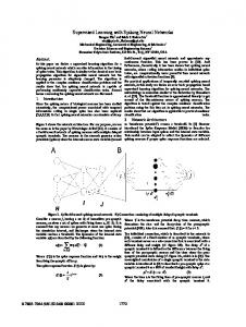
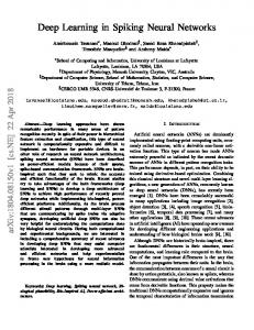
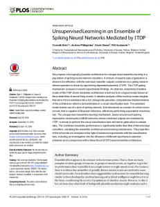
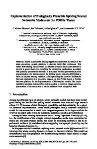
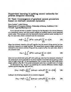
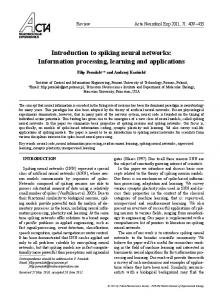
√ σ = 3 · 10−9 , α = 0.7. The step-size was β = 0.007σ 2 M (see the discussion on conditional variance in Sec. IV). Figure 1 presents simulations for various number, M , of perturbed networks. It is seen that the larger this number is, the faster learning. Fig. 3 also demonstrates variability of returns in 30 runs. Figure 2 presents simulations for different timespan, ∆, between discrete time instants. For different ∆ weights adjustment take place more often. This effect is eliminated such that the step size parameter, β, is proportional to ∆. What also changes with ∆ is volatility disturbed weights, ak , driven by ξ (3). It is seen that the larger this volatility is, the slower learning. To achieve good results, the weights ak used in learning step (5) should be similar to weights with which the network operated in the time period preceding instant k, which resulted with the current return, rk . B. Multichannel LIF, time coding, and XOR In this section a network of Leaky Integrate & Fire neurons with multichannel synapses is trained to represent the XOR logic gate. a) Neurons: A synapse is modelled as a set of N channels with different delays, dn > 0, n = 1, . . . , N . A presynaptic spike increases additively the membrane potential in the postsynaptic neuron. The membrane potential in a neuron is computed as d Cm Vm = − gL (Vm − EL ) + Iexc + Iinh dt d τexc Iexc = − Iexc dt d τinh Iinh = − Iinh dt Vm ≥ Vthresh ⇒Vm ← EL , Vm remains fixed for time tref ract , output spike. Let wi,n be the efficacy of the synapse channel n between i-th neuron and one discussed. Then, if period of dn has elapsed since last firing of neuron i, and wi,n ≥ 0, then

0

-1

-2

-3

M=1 M=2 M=4 M=7 M=12

-4

-5 0

500

1000

1500

2000

Fig. 1. LIF with frequency coding, and XOR for various number, M , of perturbed networks. Average return vs. constant input counter. Each curve averages 30 runs.

0

-1

-2

-3

d=2 d=4 d=8 d=16

-4

-5 0

500

1000

1500

2000

Fig. 2. LIF with frequency coding, and XOR for 12 perturbed networks and various timespan between discrete time moment. Average return vs. constant input counter. Each curve averages 30 runs.

0

-1

Iexc ← Iexc + wi,n . -2

Symmetrically, if wi,n < 0, then Iinh ← Iinh + wi,n .

-3

b) Network: It is built of neurons grouped in 3 layers. The first layer includes 3 neurons. Two of them translate binary input signals into moment of spike generations. The last one produces signal corresponding to binary “1”. There are 5 neurons in the second layer. They have three inputs each. The third layer of the network contains only one output neuron with 5 inputs. Weights of the network are initialized as in Sec. V-A. Dynamics of the network is simulated with Euler method and time quantization δ = 10−4 sec.

-4

average rewards in episodes

-5 0

500

1000

1500

2000

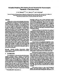
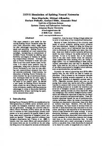
Fig. 3. LIF with frequency coding, and XOR for M = 12 perturbed networks. Average return vs. constant input counter. The curve averages 30 runs, and the bars demonstrate run-to-run variability of average returns.

335

c) Task to learn: Time coding is applied here to convey information. Network operation is episodic. At the beginning of each episode membrane potentials in the neurons are reset. Immediate occurrence of the incoming spike denotes binary “1” while its occurrence after 6ms denotes “0”. Early output spike, after 10ms, denotes “1” while late one, after 16ms, denotes “0”. The problem here is for the network to learn to represent the XOR gate. After each episode the network receives a return which is related to time distance between the moment of actual spike generation, tact , and the moment when the spike should occur, td . The return is equal to r = −(t

act

0 -1 -2 -3 -4 -5

M=1 M=2 M=4 M=7 M=15 M=24

-6 -7 -8 -9 -10 0

2000

4000

6000

8000

10000

12000

14000

−t ) . d 2

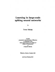
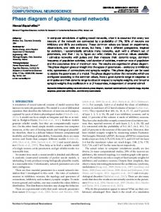
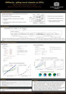
d) Simulations: An episode lasts for ∆ = 40ms. At the beginning of an episode the efficacies are selected on random according to (3), with σ = 8 · 10−10 and α = 0, and remain constant till the end of the episode, when the learning and weight perturbation for the next episode happens. At the end of each episode all neuron √ model variables are reset. The stepsize was β = 0.03σ 2 M . Figure 4 presents simulations for various number, M , of perturbed networks. It is seen that the larger this number is, the faster learning. Fig. 5 also demonstrates variability of returns in 60 runs. C. Multichannel LIF, time coding, and Wisconsin Breast Cancer In this section a network of Leaky Integrate & Fire neurons with multichannel synapses is trained on the Wisconsin Breast Cancer dataset consisting of 699 cases [11]. a) Information coding: The experiments were performed in the same way as in [1] where the SpikeProp algorithm had been introduced. Each input variable, ranging from 1 to 10, was coded using 7 neurons with Gaussian receptive fields. It’s center for neuron i was 1.8i−1.7 and standard derivation 6/5. Using these activation functions a time of spike for each input neuron was calculated — higher value of the function resulted in earlier spike, from 1ms to 10ms. Inputs that spiked 9ms or later were configured not to spike at all. Because there are two classes in WBC dataset two output neurons were used — the train signal consisted of train spike only for output neuron assigned to a category. In classification, category was determined by earliest output spike. b) Network: Because there were 9 input variables and each of them was coded using 7 neurons thus there were 63 input neurons. 15 hidden neurons were used and 2 output neurons. Neuron model was the same as for the temporal-XOR experiment. Initial weights of the network were selected randomly from the normal distribution N (5 · 10−11 , (2 · 10−11 )2 ). In 20% of randomly selected cases, a weight was reversed — it became inhibitory. c) Simulations: The dataset was divided into two subsets for cross-validation. Each training set was presented to the network for 5000 iterations (each time the 350 or 349 set was permuted). Like for the XOR experiment, an episode lasted

Fig. 4. Multichannel LIF with time coding, and XOR for various number, M , of perturbed networks. Average return vs. sample number, k. Each curve averages 60 runs. 0 -1 -2 -3 -4 -5

average rewards in episodes

-6 -7 -8 -9 -10 0

2000

4000

6000

8000

10000

12000

14000

Fig. 5. Multichannel LIF with time coding, and XOR for M = 24 perturbed networks. Average return vs. sample number, k. The curve averages 60 runs, and the bars demonstrate run-to-run variability of average returns.

for ∆ = 40ms√and parameters were: σ = 10−11 , α = 0 and β = 0.0003σ 2 M . M = 14 perturbed networks were used. The results are presented in Fig. 6. In 5000 iterations, the average accuracy for the testing set reached 90% ± 0.9. D. Discussion The simulations presented above justify the following claims concerning the presented approach: • With this method, a spiking neural network is able to learn non-trivial approximation tasks. • The method is applicable with both frequency coding and time coding. • The method can be used with any neuron model, the only prerequisite is the presence of weights and a return function. • The method is applicable both to episodic learning, and on-line, continuous learning. • Increasing number of perturbed networks decreases variance of improvement direction estimates and speeds-up learning.

336

0

[8] J. Werfel, X. Xie, and H. S. Seung, “Learning curves for stochastic gradient descent in linear feedforward networks,” Neural Computation, vol. 17, pp. 2699–2718, 2005. [9] R. S. Sutton and A. G. Barto, Reinforcement Learning: An Introduction. MIT Press, 1998. [10] H. J. Kushner and G. G. Yin, Stochastic Approximation Algorithms and Applications. Springer, 1997. [11] A. Frank and A. Asuncion, “Uci machine learning repository,” 2010.

-100 -200 -300 -400 -500

average rewards in iterations

-600 -700 0

1000

2000

3000

4000

5000

Fig. 6. Multichannel LIF with time coding, and Wisconsin Breast Cancer. Average return vs. iteration number for the test set. The curve averages 10 runs.

•

•

In case of continuous learning decreasing volatility of noise that perturb network weights increases reliability of improvement direction estimate thus speeds-up learning. The method can modify weights of neurons that are “silent” (they stopped producing spikes in response to any input spikes). The method will stop working only when all output neurons are “silent” in response to any input spikes combination and any weights perturbation caused by ξk . VI. C ONCLUSIONS

In this paper the method is presented of learning in spiking neural networks. It extends the known idea of perturbing synaptic efficacies in two directions. First, it applies perturbations that are autocorrelated in time. Second, it reduces variance of improvement direction estimate due to the use of more than just one perturbed network. The experimental study with approximation of the XOR logic gate, and reallife classification problem of Breast Cancer Wisconsin confirm that the presented approach is feasible and universal enough to work with various ways of information coding. R EFERENCES [1] S. M. Bohte, J. N. Kok, and H. L. Poutré, “Error-backpropagation in temporally encoded networks of spiking neurons,” Neurocomputing, vol. 48, pp. 17–37, 2002. [2] F. Ponulak and A. Kasinski, “Supervised learning in spiking neural networks with resume: Sequence learning, classication, and spike shifting,” Neural Computation, vol. 22, pp. 467–510, 2010. [3] I. R. Fiete and H. S. Seung, “Gradient learning in spiking neural networks by dynamic perturbation of conductances,” Physical Review Letters, vol. 97, no. 4, 2006. [4] R. V. Florian, “Reinforcement learning through modulation of spiketiming-dependent synaptic plasticity,” Neural Computation, vol. 19, pp. 1468–1502, 2007. [5] R. Williams, “Simple statistical gradient following algorithms for connectionist reinforcement learning,” Machine Learning, vol. 8, pp. 299– 256, 1992. [6] A. Dembo and T. Kailath, “Model-free distributed learning,” IEEE Transactions on Neural Networks, vol. 1, no. 1, pp. 58–70, 1990. [7] H. S. Seung, “Learning in spiking neural networks by reinforcement of stochastic synaptic transmission,” Neuron, vol. 40, pp. 1063–1073, 2003.

337