Supervised Learning with Spiking Neural Networks Jianguo Xin1 and Mark J. Embrechts2
[email protected],
[email protected] Mechanical Engineering, Aeronautical Engineering, & Mechanics1 Decision Sciences and Engineering Systems2 Rensselaer Polytechnic Institute, 110 8th St., Troy, NY 12180, USA
Since the spiking nature of biological neurons has been studied extensively, the computational power associated with temporal information coding in single spike has also been explored [3,4,6,7,9]. In fact spiking neural networks can simulate arbitrary
feed-forward sigmoidal neural network and approximate any continuous function. This has been proven in [10]. And furthermore, theoretically it has been shown that spiking neural networks, where coding information resides in individual spike trains, are computationally more powerful than neural network with sigmoidal activation functions [8]. For practical applications of temporally encoded spiking neural network, in this study we derive an error back propagation based supervised learning algorithm for spiking neural networks. The methodology is somewhat similar to the derivation by Rumelhart et al. [12]. The threshold function is approximated linearly to get around of the discontinuous nature of spiking neurons. The algorithm is tested against the complex nonlinear classification problem using the Iris data set in spiking neural networks. The results show that our algorithm is applicable to practical nonlinear classification tasks.
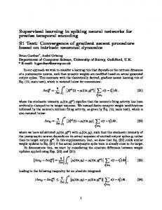
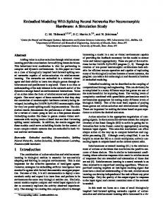
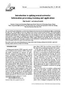
Figure 1 shows the network architecture. For our purpose, we use the same as in the paper by Natschlager & Ruf [11]. It consists of a feed-forward network of spiking neurons with multiple delayed synaptic terminals. The neurons in the network generate action potentials (spikes) when the internal neuron state variable (termed
as ‘membrane potential’) crosses a threshold. In [5] Gerstner introduced the Spike Response Model (SRM) to describe the relationship between input spikes and the internal state variable. This model can be adapted to reflect the dynamics of different spiking neurons if proper spike response functions are selected.
Abstract In this paper we derive a supervised learning algorithm for a spiking neural network which encodes information in the timing of spike trains. This algorithm is similar to the classical error back propagation algorithm for sigmoidal neural network but the learning parameter is adaptively changed. The algorithm is applied to the complex nonlinear classification problem and the results show that the spiking neural network is capable of performing nonlinearly separable classification tasks. Several issues concerning the spiking neural network are discussed.
1.
Introduction
2.
Network Architecture
Figure 1. A) Feed-forward spiking neural network B) Connection consisting of multiple delayed synaptic terminals Consider a neuron j, having a set Dj of immediate pre-synaptic Where τ is the membrane potential decay time constant, which neurons, receives a set of spikes with firing times ti, i ∈ Dj. It is determines the rise- and the decay-time of the postsynaptic assumed that any neuron can generate at most one spike during potential (PSP). Also it is assumed that ε (t) = 0 for t < 0. the simulation interval, and discharges when the internal state variable reaches a threshold. The dynamics of the internal state The individual connection, which is described in the network in [11], consists of a fixed number of m synaptic terminals, where variable xi(t) are described by the following function: each terminal serves as a sub-connection that is associated with a different delay and weight (cf. figure 1B). The delay dk of a wij ε (t - ti) xi(t) = (1) synaptic terminal k is defined as the difference between the firing i∈Dj time of the pre-synaptic neuron and the time when the postWhere ε (t) is the spike response function and wij is the weight synaptic potential starts rising (cf. figure 2A, which is in [2]). The un-weighted contribution of a single synaptic terminal to the state describing the synaptic efficacy. variable is introduced in [2] to described a pre-synaptic spike at a The spike response function ε (t) is given by: synaptic terminal k as a PSP of standard height with delay dk:
å
ε (t) =
t 1-t/ τ e τ
0-7803-7044-9/01/$10.00 ©2001 IEEE
(2)
yik = ε (t – ti - dk)
(3)
Where the time ti is the firing time of pre-synaptic neuron i, and dk the delay associated with the synaptic terminal k.
1772
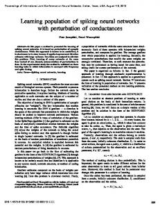
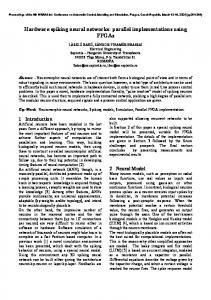
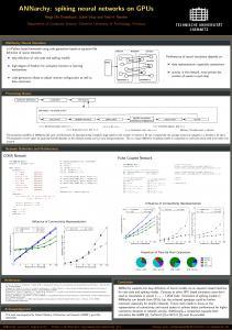
Figure 2. Connections in a feed-forward spiking neuron network: A. Single synaptic terminal: the delayed pre-synaptic potential is weighted by the synaptic efficacy to obtain the post-synaptic potential. B. Two multi-synapse connections: weighted input is summed at the target neuron. Now consider the multiple synapses per connection. From Where k is the weight associated with synaptic terminal k (cf. wij equation (1) and combining equation (2), the state variable xj of neuron j receiving input from all neurons i is then described as the figure 2B). The firing time tj of neuron j is defined as the first weighted sum of the pre-synaptic contributions: time when the state variable crosses the threshold θ : xj(t) ≥ θ . m The threshold θ is a constant and fixed for all neurons in the k k xj(t) = (4) wij yi (t ) network.
åå
Dj k =1 Error Back Propagation Algorithm i∈
To minimize the objective function in equation (5), we need to optimize the weight who between each separate connection k of Consider a fully connected feed-forward neural network with layers identified as I (Input), H (Hidden) and O (Output). We will the synaptic terminal, e.g. wkho . Therefore, for the back derive an algorithm based on error back propagation. It should be k noted that the derived algorithm can be applied to networks with propagation rule, the weight correction ∆ who needs to be more than one hidden layer as well. calculated: The learning scheme is teacher forcing, that is to learn a set of
3.
∆ wkho
t
target firing times, denoted as { t o }, at the output neurons
=
−η
∂E ∂ wkho
(6)
o ∈ O for a given set of input patterns {P[t1...ti]}, where k P[t1...ti] defines a single input pattern described by single spike Where η is the learning parameter and who is the weight of train for each neuron i ∈ I . The objective function to be connection k from neuron h to neuron o. The derivative on the right hand of equation (6) can be expressed as follows using the optimized is the least squares error function: chain rule and considering the fact that to is a function of xo, E= t
1 å ( tao - tot ) 2 2 o∈O
which
(5)
depends
on
the
weights
k
who :
a
Where { t o } and { t o } are the target spike train and spiking neural network actual output spike train, respectively. approximated by a linear function of t and thus we express to as a
∂E ∂E a ∂to a ∂E a ∂to a = (t o ) (t o ) = (t o ) (t o ) ∂ wkho ∂to ∂to ∂xo(t) ∂ wkho
∂xo (t ) a (t o ) ∂ wkho
function of the threshold post-synaptic input xo(t) around t =
In such a small region, the threshold function can be
(7)
approximated as
In the above expression we make an assumption just as in [2]: for a small enough region around
a
to .
t = t ao , the function xo can be
1773
δto ( xo ) = −δxo(to ) / λ .
∂to ∂xo(t )
is the
λ is the local ∂xo (t ) a λ= (t o ) . ∂t −1 −1 = = λ ∂xo(t ) ( a ) to ∂t
derivative of the inverse function of xo(t) and derivative of xo(t) with respect to t, e.g.
∂to a (t o ) ∂xo(t)
=
∂to ( xo ) ∂xo(t )
xo=θ
=
−1
å wlho h ,l
∂ y lh (t ) a (t o ) ∂t
∂ t oa
= t oa − t to
∂ wkho
=y
k h
(9)
(t ) a o
=
∂ t oa
δh =
, and the same holds for similar expressions.
∂ t ah
∂E
∂ t ah ∂xh(t ah )
å∂ j∈Dh
t aj ∂xj (t aj ) ∂ t ah ∂xh (t ah )
=
(10)
å δj j∈Dh
k h
y (t oa ) ⋅ (t to − t oa ) −η l a l ∂ y h (t o ) åh∈D ålwho ∂ t oa
=
∂ t aj ∂xj (t aj ) ∂ t ah
∂E
∂xj (t aj ) ∂ t ah ∂ t ah ∂xh(t ah )
(15)
where Dh denotes the set of immediate successive neurons in layer O connected to neuron h.
Now combine the above results, for equation (6) we have:
∆ wkho (t oa )
∂xo(t oa )
and
(11) In the above expression we expand the derivative
o
∂E ∂ t oa = ∂ t oa ∂xo(t oa )
(t to − t oa ) l a l ∂ y h (t o ) åh∈Do ålwho ∂ t oa
(12)
∂ w kho
= y kh (t oa)δo
∂xj (t aj) ∂ t ah
(13)
=
− η y kh (t oa)δo
∂ t ah
has been calculated in (8), while for
=
∂ åå wljk ylk (t aj) l∈H
k
∂ t ah
∂ y kh (t aj) = åw ∂ t ah k k hj
(16)
(14)
Now we consider the error back propagation in the hidden layer. For h ∈ H , the generalized delta error in layer H is defined with actual firing times
in
:
∂xj (t aj)
And finally we have:
∆ wkho
∂ t ah ∂xh (t ah )
The term
Using expression (12), equation (7) can be written as:
∂E
∂E (t ah ) ∂ t ah
terms of the weighted error contributed to the subsequent layer O. Also the chain rule is used for the case t = th.
For expression simplicity, we define δo :
δo =
∂xo (t ) a (t o ) ∂t
Clearly the above assumption is related to the learning parameter and only true when it is small. This will be verified in the later section of our study.
From expression in equation (4) and apply it for the output layer, we derive:
∂xo(t oa )
We will not differentiate between the expression
(8)
According to the objective function, equation (5), the first factor in the right hand of (7), the derivative of E with respect to to, is:
∂E (t oa )
Using the above information, we can express part of factor in (7) as follows:
Hence, k
∂ y h (t aj ) } ∂ t ah j∈D k δh = l a l ∂ yi (t h ) wih åå ∂ t ah i∈D l
å δj{å wkhj
a
th :
h
(17)
h
According to the expression of (14), (15), (16) and (17), the weight update rule for a hidden layer amounts to:
1774
∆ wihk
Just as for the classical error back-propagation algorithms, the weight update formula (18) can be generalized to a network with multiple hidden layers. The delta-error at hidden layer h is calculated by back propagating the error from the delta-error at higher layer h + 1.
=
− η yik (t ah )δh = −η ∂ ykh (t aj ) } y t å {δj å w ∂ t ah j k l a l ∂ yi (t h ) åå wih ∂ t ah i∈Dh l k a i ( h)
4.
k hj
(18)
Momentum and Adaptive Learning Parameter Scheme
In [2] it was reported that no convergence failures of the SpikeProp were found for the data sets being studied, but there might exist local minima in some optimization problem, e.g. in the error back propagation algorithm above. To improve convergence and get around of local minimum, a momentum term is added to the weight update procedure, hopefully making the algorithm more robust. Another issue concerning the error back propagation algorithm is the computation load, or convergence speed. Also convergence rate, which is related to the learning paratemter, was found slow for the SpikeProp algorithm in [2], especially for large data sets. Large learning parameter means that the step size is too big for the weight update per iteration and the objective function might not be able to reach its global minima. The optimization procedure might go into the cyclic state. Thus large value of learning parameter usually associates with bad classification results. On the other hand, if the learning parameter is too small, which means we are too conservative in our choice, then it might need much more iterations to reach the global minima, hence the computation time will be longer and the convergence rate is slow. This is the motivation of our adaptive learning parameter scheme – selecting the learning parameter in some optimal sense to speed up the convergence rate. In our algorithm the learning parameter is adjusted dynamically following the QuickProp approach. The basic idea is when the weight correction sign is positive, it increases, whereas decreases when the error sign is negative. So the weight update formula in our algorithm is as follows: k +1 k k k −1 w ji = w ji + η k δ ji + α∆ w ji
Where:
ηk
∆ wkji−1
the previous iteration.
Encoding Input Variables
6.
Experimental Results with Iris Dataset
In this paper we want to concentrate on the Iris dataset and make a thorough study of our algorithm with spiking neural networks against this dataset. The Iris dataset consists of three classes, two of which are not linearly separable, thus provides a good practical problem for our algorithm. The dataset contains 150 data samples with 4 continuous input variables. As in [2], we employ 12 neurons with Gaussian receptive fields to encode each of the 4 input variables, and divide the dataset into training and testing set, each of which has half (75) of the sample numbers.
6.1 Spiking Neural Network Structure
The first thing to be settled is the network structure, namely how is the many hidden layers and how many neurons in each layer. This is is the weight correction in ad hoc and depends on specific problem. For comparison, we also adopted the general one hidden layer structure. The network structures we tried are 50x10x3 and 50x20x3 with static fixed by Population Coding learning parameters 0.05. The results are given below.
is the learning parameter per iteration,
momentum parameter, and
5.
(19)
For practical classification problems, the input variables are normally in continuous form. So the first problem when we use spiking neural network is how to encode input variables into temporal spike train. Basically there are two schemes. The first is by using increasingly small temporal differences and the second is by distributing the input over multiple neurons. There is a side effect with the first scheme: The increased temporal resolution for the input variables will increase the computational load on the spiking neural network. Another concern with this approach, which has been pointed out in [2], is that it is not biologically plausible. So in our algorithm we adopt the second one population coding. The basic idea is employing arrays of receptive fields (RF’s), which enables the representation of continuous input variables by a pool of neurons with graded and overlapping sensitivity profiles, e.g. Gaussian activation functions. This encoding scheme is biologically more plausible. The highly stimulated neurons are associated with early firing times and less stimulated neurons with later (or no) firing times. Detailed information on population coding is given in [1,2,4,13,14].
α
Network Iterations Structure vs. 500 1000 1100 1200 1300 1400 1500 1600 % of correct classification 50x10x3(1) 94.67 93.33 94.67 94.67 94.67 96.00 97.33 94.67 50x20x3(2) 89.33 94.67 97.33 94.67 94.67 97.33 96.00 94.67 Table 1. Testing classification results vs. different network structure, static learning parameter η = 0.05 The results in table 2 show that the network with more neurons learns comparatively slowly at first. This is due to the more weights to be adjusted. Note that the weights for the 2nd network structure (50x20x3) has doubled compared with the 1st structure (50x10x3). With further iterations, it learns more quickly than the one with less neurons. In our case, classification result has reached the maximum value of 97.33% after 1100 and 1500 iterations, respectively, for the two network structures. This does not necessarily mean the total computation time in the 2nd case is less than the 1st case. In fact, with more weights to be adjusted, for each iteration, the computation load is much heavier in the 2nd
structure than the 1st one. This results in more computation time to reach the global minima for the 2nd structure. So in our network, we adopt the 1st smaller compact structure rather than the 2nd one.
6.2 Momentum and Its Effect on the Classification Results The next comparative study we made is the momentum term in the weight update equation (19). In our study we found that by adding the momentum term in our algorithm, the classification results for the testing dataset seem to
1775
be somewhat oscillating even if the momentum parameter α is small, which means that it deteriorates the classification results. Another issue concerning the momentum term is it requires more storage when the weight is updated. The previous weight difference has to be saved for the current step. This might be trivial if the data set is small and the computer memory is high enough. But for practical complex nonlinear classification problem where the data set is very large and which entails more weights, the storage will become an important issue when the momentum term is added to the weight adaptation. The computation load for weight update will be higher as well though not as severe as the storage problem. So in our further study, the momentum parameter is set to zero.
6.3 Static Learning Parameter η
empirically by trial and error. The results of different cases we have tried are given in table 1. From the results shown in table 1, we can see that with small learning parameter, which is in the range of [0.01, 0.05], the classification results are pretty good – the number of wrongly classified data sample varies between 2 and 5 out of 75 testing data samples for all the iteration 500 till 1600, and the percentage of correct classification is between 93.33% and 97.33%. If the learning parameter is beyond 0.1, the results are rather bad after 500 iterations - the percentage is 33.33% and 34.67%, respectively for the value of 0.1 and 0.5. After further training, the results improve much better – it reaches the maximum percentage 97.33% after 1200 and 1000 iterations for the value of 0.1 and 0.5, respectively. So in our algorithm, we adaptively adjust the learning parameter η and let it varies between 0.001
Another important parameter to be identified is the learning and 0.05. parameter η . There is no way to decide it theoretically. We can The above results also confirm the former assumption in section 3 obtain the maximum allowable static value of learning parameter of this study. Iteration vs. Learning 500 1000 1100 1200 1300 1400 1500 1600 % of correct Parameter η classification 0.01
Training Testing Training Testing Training Testing Training Testing
0.05 0.1 0.5
97.33 97.33 97.33 97.33 97.33 97.33 93.33 96.00 97.33 94.67 96.00 97.33 97.33 97.33 96.00 96.00 97.33 96.00 94.67 93.33 94.67 94.67 94.67 96.00 33.33 76.00 89.33 96.00 96.00 96.00 33.33 74.67 92.00 97.33 93.33 94.67 36.00 96.00 96.00 94.67 97.33 97.33 34.67 97.33 96.00 96.00 96.00 97.33 Table 2. Classification results vs. static learning parameter η
6.4 Results of the Adaptive Learning Parameter Scheme
97.33 97.33 97.33 97.33 96.00 97.33 97.33 97.33
97.33 94.67 97.33 94.67 92.00 84.00 97.33 96.00
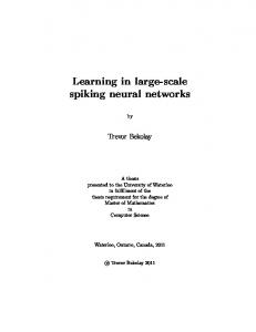
Adaptive vs. Non-adaptve Learing Parameter, Case 2 100
Percentaqge of Classification Results (%)
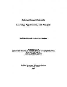
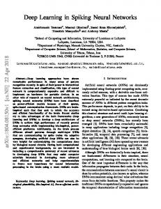
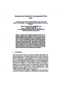
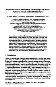
In this section, we present the results of our study with adaptive learning parameter scheme. We tested our adaptive algorithm in two cases. For the first case, the initial learning parameter η is 0.005, and the maximum value is limited to 0.05. The classification results are given figure 3. From figure 1,we can see that the adaptive learning scheme learns much faster for the first 200 iterations, the classification rate reaches 89.33% (32.67% higher) at 100 iterations; one of its local peak, 93.33% (6.67% higher) at 120 iterations. After 450 iterations, both schemes reach their highest percentage 97.33%. As our second case, the initial learning parameter η is 0.001, and the maximum value is limited to 0.01. The classification results are given in figure 4.
90
80
70
60 Adaptive Non-adaptve
50
40
Adaptive vs. Non-adaptve Learing Parameter, Case 1
Percentaqge of Classification Results (%)
100
30 100
95
90
85 Adaptive Non-adaptve
80
75
70
65 100
150
200
250 300 Iterations
350
400
450
Figure 3. Testing classification results: adaptive vs. non-adaptive learning scheme, case 1.
200
300
400 Iterations
500
600
Figure 4. Testing classification results: Adaptive vs. Non-adaptive learning scheme, case 2. The advantage of the adaptive learning scheme is more pronounced in the second case. From figure 4, we can see that the adaptive learning scheme learns much faster for the first 280 iterations, the classification rate reaches one of its local peak 89.33% (22.67% higher) during this period. For most of the iterations we sampled, the correct classification results are much higher for the adaptive case than the non-adaptive one. After 650 iterations, both schemes reach their highest percentage 96.00% vs. 94.67% (1.33% higher), respectively. From these two cases, we conclude that the adaptive learning scheme learns faster than the non-adaptive one, and the correct classification percentage is better or comparable to corresponding case. We believe that for more complex nonlinear classification problem with very large data sets, the importance of adaptive
1776
700
learning parameter scheme will be more significant in terms of momentum are both set to 0.25. The results of running the computation time and classification rate. MetaNeuron along with the ones in [2] are shown in table 5. 6.5 Comparison Results of Different Learning Algorithm From table 5, we can see that for the Iris dataset, in terms of the iteration numbers to obtain the optimal classification results, our on Iris Dataset adaptive learning parameter scheme seems to be somewhat more Finally we did some but not thorough comparison between preferable than the rest ones. Regarding the maximum correct several back propagation algorithms with different neural network classification rate, our scheme is equally as good as MetaNeuron structure on the Iris dataset. and better than the Matlab back propagation “TRAINLM” routine First we run the iris dataset against our in-house software - and the SpikeProp which implements error back propagation MetaNeuron ver. 6.11. This is a thoroughly designed software algorithm using spiking neural networks. implementing the back propagation learning algorithm using the So the overall performances of our algorithm for the Iris dataset sigmoidal function with ANN. By trial and error, the proper are better than the other three that have been reported or studied. network structure for using MetaNeuron is 4x10x10x3, e.g. there are two hidden layers. The parameters for learning and Iris Dataset Maximum Algorithm Inputs Hidden Outputs Iterations Classification Rate SpikeProp 50 10 3 1,000 96.2% Matlab BP 50 10 3 3,750 95.8% MetaNeuron 4 10x10 3 1,500 97.33% QuickProp 50 10 3 450 97.33% Table 3. Classification result of iris dataset using different back propagation algorithms We should point out that while testing our algorithm against the Iris dataset, we identified the over-training phenomenon, which is understandable – All error back propagation algorithm has this inherent shortcoming.
7.
Conclusions
This study presents an adaptive learning algorithm for spiking neural network based on back propagating the output temporal error. To enhance the robustness of the algorithm when dealing with complex classification problem, a momentum term is considered in the algorithm and its effect on the classification results is studied. The adaptive learning parameter scheme is thoroughly studied against the Iris data set and the results demonstrate that the algorithm for the spiking neural network is successfully capable of solving practical nonlinear complex classification problem.
Acknowledgements The first author would like to thank Dr. Bohte at the National Research Institute for Mathematics and Computer Science in the Netherlands for the help regarding some contents in the paper, and Dr. Choe in the Department of Computer Sciences, The University of Texas at Austin for the many stimulating discussions about spiking neural networks.
References [1] P. Baldi and W. Heiligengerg, How sensory maps could enhance resolution through ordered arrangements of broadly tuned receivers, Biol. Cybern. 59(1988) 313-318. [2] S.M. Bohte, J.N. Kok, and H. La Poutre, ErrorBackpropagation in Temporally Encoded Networks of Spiking Neurons, in Proceedings of ESANN'2000. [3] Y. Choe, R. Miikkulainen, Self-Organization and Segmentation in a Laterally Connected Orientation Map of Spiking Neurons. Neurocomputing volume 21, 139-157, 1998.
[4] A.K. Engel, P. Konig, A.K. Kreiter, T.B. Schillen, and W. Singer, Temporal coding in the visual cortex: new vistas on integration in the nervous system, Trends Neurosci. 15(1992) 218-226. [5] W. Gerstner, Time structure of the activity in neural network models, Phys Rev E, 51(1995) 738-758. [6] W. Gerstner, Spiking neurons, in W. Maass and C. Bishop, editors, Pulsed Neural Networks (MIT Press, Cambridge, 1999). [7] W. Gerstner, R. Kempter, J.L. van Hemmen, and H. Wagner, A neuronal learning rule for sub-millisecond temporal coding, Nature, 383(1996) 76-78. [8] W. Maass, Lower bounds for the computational power of networks of spiking neurons, Neural Comp., 8(1996) 1-40. [9] W. Maass, Paradigms for computing with spiking neurons, in L. van Hemmen, editor, Models of Neural Networks, volume 4, (Spinger Brelin, 1999). [10] W Maass, Fast sigmoidal networks via spiking neurons, Neural Comp., 9(1997)279-304. [11] T. Natschlager and B. Ruf, Spatial and temporal pattern analysis via spiking neurons, Network: Comp. In Neural Syst., 9(1998) 319-332. [12] D.E. Rumelhart, G.E. Hilton, and R.J. Williams, Learning representations by back-propagating errors, Nature, 323(1986) 533-536. [13] M.N. Shadlen and W.T. Newsome, The variable discharge of cortical neurons: implications for connectivity, computation and information coding, J. Neuronsci, 18(1998) 3870-3896. [14] K.-C. Zhang, I. Ginzburg, B.Ll McNaughton, Interpreting neuronal population activity by reconstruction: Unified framework with application to hippocampal place cells, J. Neurophys, 79(1998) 1017-10
1777