Learning rates for the risk of kernel based quantile regression ... - arXiv

arXiv:1405.3379v1 [stat.ML] 14 May 2014

Learning rates for the risk of kernel based quantile regression estimators in additive models† Andreas Christmann1 and Ding-Xuan Zhou2 1 University of Bayreuth, Germany 2 City University of Hong Kong, China May 11, 2014 Abstract Additive models play an important role in semiparametric statistics. This paper gives learning rates for regularized kernel based methods for additive models. These learning rates compare favourably in particular in high dimensions to recent results on optimal learning rates for purely nonparametric regularized kernel based quantile regression using the Gaussian radial basis function kernel, provided the assumption of an additive model is valid. Additionally, a concrete example is presented to show that a Gaussian function depending only on one variable lies in a reproducing kernel Hilbert space generated by an additive Gaussian kernel, but does not belong to the reproducing kernel Hilbert space generated by the multivariate Gaussian kernel of the same variance.

Key words and phrases. Additive model, kernel, quantile regression, semiparametric, rate of convergence, support vector machine.

1

Introduction

Additive models [30, 9, 10] provide an important family of models for semiparametric regression or classification. Some reasons for the success of addi† The work by A. Christmann described in this paper is partially supported by a grant of the Deutsche Forschungsgesellschaft [Project No. CH/291/2-1]. The work by D. X. Zhou described in this paper is supported by a grant from the Research Grants Council of Hong Kong [Project No. CityU 104710].

1

tive models are their increased flexibility when compared to linear or generalized linear models and their increased interpretability when compared to fully nonparametric models. It is well-known that good estimators in additive models are in general less prone to the curse of high dimensionality than good estimators in fully nonparametric models. Many examples of such estimators belong to the large class of regularized kernel based methods over a reproducing kernel Hilbert space H, see e.g. [21, 38]. In the last years many interesting results on learning rates of regularized kernel based models for additive models have been published when the focus is on sparsity and when the classical least squares loss function is used, see e.g. [18], [1], [17], [19], [22], [33] and the references therein. Of course, the least squares loss function is differentiable and has many nice mathematical properties, but it is only locally Lipschitz continuous and therefore regularized kernel based methods based on this loss function typically suffer on bad statistical robustness properties, even if the kernel is bounded. This is in sharp contrast to kernel methods based on a Lipschitz continuous loss function and on a bounded loss function, where results on upper bounds for the maxbias bias and on a bounded influence function are known, see e.g. [4] for the general case and [3] for additive models. Therefore, we will here consider the case of regularized kernel based methods based on a general convex and Lipschitz continuous loss function, on a general kernel, and on the classical regularizing term λk · k2H for some λ > 0 which is a smoothness penalty but not a sparsity penalty, see e.g. [36, 37, 23, 32, 6, 26, 11, 7]. Such regularized kernel based methods are now often called support vector machines (SVMs), although the notation was historically used for such methods based on the special hinge loss function and for special kernels only, we refer to [35, 2, 5]. In this paper we address the open question, whether an SVM with an additive kernel can provide a substantially better learning rate in high dimensions than an SVM with a general kernel, say a classical Gaussian RBF kernel, if the assumption of an additive model is satisfied. Our leading example covers learning rates for quantile regression based on the Lipschitz continuous but non-differentiable pinball loss function, which is also called check function in the literature, see e.g. [16] and [15] for parametric quantile regression and [24], [34], and [28] for kernel based quantile regression. We will not address the question how to check whether the assumption of an additive model is satisfied because this would be a topic of a paper of its own. Of course, a practical approach might be to fit both models and compare their risks evaluated for test data. For the same reason we will also not cover sparsity. Consistency of support vector machines generated by additive kernels for 2

additive models was considered in [3]. In this paper we establish learning rates for these algorithms. Let us recall the framework with a complete separable metric space X as the input space and a closed subset Y of R as the output space. A Borel probability measure P on Z := X ×Y is used to model the learning problem and an independent and identically distributed sample Dn = {(xi , yi )}ni=1 is drawn according to P for learning. A loss function L : X × Y × R → [0, ∞) is used to measure the quality of a prediction function f : X → R by the local error L(x, y, f (x)). Throughout the paper we assume that L is measurable, L(x, y, y) = 0, convex with respect to the third variable, and uniformly Lipschitz continuous satisfying sup |L(x, y, t) − L(x, y, t0 )| ≤ |L|1 |t − t0 |

∀t, t0 ∈ R

(1.1)

(x,y)∈Z

with a finite constant |L|1 ∈ (0, ∞). Support vector machines (SVMs) considered here are kernel-based regularization schemes in a reproducing kernel Hilbert space (RKHS) H generated by a Mercer kernel k : X × X → R. With a shifted loss function L∗ : X × Y × R → R introduced for dealing even with heavy-tailed distributions as L∗ (x, y, t) = L(x, y, t) − L(x, y, 0), they take the form fL,Dn ,λ where for a general Borel measure ρ on Z, the function fL,ρ,λ is defined by Z  2 fL,ρ,λ = arg min RL∗ ,ρ (f ) + λkf kH , RL∗ ,ρ (f ) = L∗ (x, y, f (x)) dρ(x, y), f ∈H

Z

(1.2) where λ > 0 is a regularization parameter. The idea to shift a loss function has a long history, see e.g. [14] in the context of M-estimators. It was shown in [4] that fL,ρ,λ is also a minimizer of the following optimization problem involving the original loss function L if a minimizer exists: Z  2 L(x, y, f (x)) dρ(x, y) + λkf kH . min (1.3) f ∈H

Z

The additive model we consider consists of the input space decomposition X = X1 × . . . × Xs with each Xj a complete separable metric space and a hypothesis space F = {f1 + . . . + fs : fj ∈ Fj , j = 1, . . . , s} ,

(1.4)

where Fj is a set of functions fj : Xj → R each of which is also identified as a map (x1 , . . . , xs ) 7−→ fj (xj ) from X to R. Hence the functions from F take the additive form f (x1 , . . . , xs ) = f1 (x1 ) + . . . + fs (xs ). We mention, that there is strictly speaking a notational problem here, because in the previous 3

formula each quantity xj is an element of the set Xj which is a subset of the full input space X , j = 1, . . . , s, whereas in the definition of sample Dn = {(xi , yi )}ni=1 each quantity xi is an element of the full input space X , where i = 1, . . . , n. Because these notations will only be used in different places and because we do not expect any misunderstandings, we think this notation is easier and more intuitive than specifying these quantities with different symbols. The additive kernel k = k1 + . . . + ks is defined in terms of Mercer kernels kj on Xj as k ((x1 , . . . , xs ), (x01 , . . . , x0s )) = k1 (x1 , x01 ) + . . . + ks (xs , x0s ). It generates an RKHS H which can be written in terms of the RKHS Hj generated by kj on Xj corresponding to the form (1.4) as H = {f1 + . . . + fs : fj ∈ Hj , j = 1, . . . , s} with norm given by kf k2H =

min

f =f1 +...+fs f1 ∈H1 ,...,fs ∈Hs

kf1 k2H1 + . . . + kfs k2Hs .

The norm of f := f1 + . . . + fs satisfies kf1 + . . . + fs k2H ≤ kf1 k2H1 + . . . + kfs k2Hs ,

f1 ∈ H1 , . . . , fs ∈ Hs . (1.5)

To illustrate advantages of additive models, we provide two examples of comparing additive with product kernels. The first example deals with Gaussian RBF kernels. All proofs will be given in Section 4. Example 1. Let s = 2, X1 = X2 = [0, 1] and X = [0, 1]2 . Let σ > 0 and   |u − v|2 , u, v ∈ [0, 1]. k1 (u, v) = k2 (u, v) = exp − σ2 The additive kernel k ((x1 , x2 ), (x01 , x02 )) = k1 (x1 , x01 ) + k2 (x2 , x02 ) is given by     |x1 − x01 |2 |x2 − x02 |2 0 0 k ((x1 , x2 ), (x1 , x2 )) = exp − + exp − . (1.6) σ2 σ2 Furthermore, the product kernel k Π ((x1 , x2 ), (x01 , x02 )) = k1 (x1 , x01 ) · k2 (x2 , x02 ) is the standard Gaussian kernel given by   |x1 − x01 |2 + |x2 − x02 |2 Π 0 0 (1.7) k ((x1 , x2 ), (x1 , x2 )) = exp − σ2 ! |(x1 , x2 ) − (x01 , x02 )|2 = exp − . (1.8) σ2 4

Define a Gaussian function f on X = [0, 1]2 depending only on one variable by   |x1 |2 . (1.9) f (x1 , x2 ) = exp − 2 σ Then f ∈ H but f 6∈ HkΠ ,

(1.10)

where HkΠ denotes the RKHS generated by the standard Gaussian RBF kernel kΠ. The second example is about Sobolev kernels. Example 2. Let 2 ≤ s ∈ N, X1 = . . . = Xs = [0, 1] and X = [0, 1]s . Let  W 1 [0, 1] := u ∈ L2 ([0, 1]); Dα u ∈ L2 ([0, 1]) for all |α| ≤ 1 be the Sobolev space consisting of all square integrable univariate functions whose derivative is also square integrable. It is an RKHS with a Mercer kernel k ∗ defined on [0, 1]2 . If we take all the Mercer kernels k1 , . . . , ks to be k ∗ , then Hj = W 1 [0, 1] for each j. The additive kernel k is also a Mercer kernel and defines an RKHS  H = H1 + . . . + Hs = f1 (x1 ) + . . . + fs (xs ) : f1 , . . . , fs ∈ W 1 [0, 1] . However, the multivariate Sobolev space W 1 ([0, 1]s ), consisting of all square integrable functions whose partial derivatives are all square integrable, contains discontinuous functions and is not an RKHS. Denote the marginal distribution of P on Xj as PXj . Under the assumption that Hj ⊂ Fj ⊂ L1 (PXj ) for each j and that Hj is dense in Fj in the L1 (PXj )-metric, it was proved in [3] that RL∗ ,P (fL,Dn ,λ ) → R∗L∗ ,P,F := inf RL∗ ,P (f ) f ∈F

(n → ∞)

in probability as long as λ = λn satisfies limn→∞ λn = 0 and limn→∞ λ2n n = ∞. The rest of the paper has the following structure. Section 2 contains our main results on learning rates for SVMs based on additive kernels. Learning rates for quantile regression are treated as important special cases. Section 3 contains a comparison of our results with other learning rates published recently. Section 4 contains all the proofs and some results which can be interesting in their own.

5

2

Main results on learning rates

In this paper we provide some learning rates for the support vector machines generated by additive kernels for additive models which helps improve the quantitative understanding presented in [3]. The rates are about asymptotic behaviors of the excess risk RL∗ ,P (fL,Dn ,λ ) − R∗L∗ ,P,F and take the form O(m−α ) with α > 0. They will be stated under three kinds of conditions involving the hypothesis space H, the measure P , the loss L, and the choice of the regularization parameter λ.

2.1

Approximation error in the additive model

The first condition is about the approximation ability of the hypothesis space H. Since the output function fL,Dn ,λ is from the hypothesis space, the learning rates of the learning algorithm depend on the approximation ability of the hypothesis space H with respect to the optimal risk R∗L∗ ,P,F measured by the following approximation error. Definition 1. The approximation error of the triple (H, P, λ) is defined as  D(λ) = inf RL∗ ,P (f ) − R∗L∗ ,P,F + λkf k2H , λ > 0. (2.1) f ∈H

To estimate the approximation error, we make an assumption about the minimizer of the risk (2.2) fF∗ ,P = arg inf RL∗ ,P (f ). f ∈F

For each j ∈ {1, . . . , s}, define the integral operator Lkj : L2 (PXj ) → L2 (PXj ) associated with the kernel kj by Z Lkj (f )(xj ) = kj (xj , uj )f (uj )dPXj (uj ), xj ∈ Xj , f ∈ L2 (PXj ). Xj

We mention that Lkj is a compact and positive operator on L2 (PXj ). Hence we can find its normalized eigenpairs ((λj,` , ψj,` ))`∈N such that (ψj,` )`∈N is an orthonormal basis of L2 (PXj ) and λj,` → 0 as ` → ∞. Fix r > 0. Then we can define the r-th power Lrkj of Lkj by Lrkj

X `



cj,` ψj,` =

X

cj,` λrj,` ψj,` ,

∀(cj,` )`∈N ∈ `2 .

`

This is a positive and bounded operator and its range is well-defined. The assumption fj∗ = Lrkj (gj∗ ) means fj∗ lies in this range. 6

Assumption 1. We assume fF∗ ,P ∈ L∞ (PX ) and fF∗ ,P = f1∗ + . . . + fs∗ where for some 0 < r ≤ 21 and each j ∈ {1, . . . , s}, fj∗ : Xj → R is a function of the form fj∗ = Lrkj (gj∗ ) with some gj∗ ∈ L2 (PXj ). The case r = 21 of Assumption 1 means each fj∗ lies in the RKHS Hj . A standard condition in the literature (e.g., [25]) for achieving decays of the form D(λ) = O(λr ) for the approximation error (2.1) is fF∗ ,P = Lrk (g ∗ ) with some g ∗ ∈ L2 (PX ). Here the operator Lk is defined by Z X s  0 Lk (f )(x1 , . . . , xs ) = kj (xj , xj )) f (x01 , . . . , x0s )dPX (x01 , . . . , x0s ). (2.3) X

j=1

In general, this cannot be written in an additive form. However, the hypothesis space (1.4) takes an additive form F = F1 + . . . + Fs . So it is natural for us to impose an additive expression fF∗ ,P = f1∗ + . . . + fs∗ for the target function fF∗ ,P with the component functions fj∗ satisfying the power condition fj∗ = Lrkj (gj∗ ). The above natural assumption leads to a technical difficulty in estimating the approximation error: the function fj∗ has no direct connection to the marginal distribution PXj projected onto Xj , hence existing methods in the literature (e.g., [25]) cannot be applied directly. Note that on the product space Xj × Y, there is no natural probability measure projected from P , and the risk on Xj × Y is not defined. Our idea to overcome the difficulty is to introduce an intermediate function fj,λ . It may not minimize a risk (which is not even defined). However, it approximates the component function fj∗ well. When we add up such functions f1,λ +. . .+fs,λ ∈ H, we get a good approximation of the target function fF∗ ,P , and thereby a good estimate of the approximation error. This is the first novelty of the paper. Theorem 1. Under Assumption 1, we have D(λ) ≤ Cr λr

∀ 0 < λ ≤ 1,

(2.4)

where Cr is the constant given by s   X ∗ ∗ 2 Cr = |L|1 kgj kL2 (PXj ) + kgj kL2 (PX ) . j

j=1

2.2

Special bounds for covering numbers in the additive model

The second condition for our learning rates is about the capacity of the hypothesis space measured by `2 -empirical covering numbers. 7

Definition 2. Let G be a set of functions on Z and z = {z1 , · · · , zm } ⊂ Z. For every  > 0, the covering number of G with respect to the empirical
2 1/2  P is defined as metric d2,z , given by d2,z (f, g) = m1 m i=1 f (zi ) − g(zi ) ` n o [ N2,z (G, ) = inf ` ∈ N : ∃{fi }`i=1 ⊂ G such that G = {f ∈ G : d2,z (f, fi ) ≤ } i=1

and the `2 -empirical covering number of G is defined as   N (G, ) = sup sup N2,z G,  . m∈N z∈Z m

p P Assumption 2. We assume κ := sj=1 supxj ∈Xj kj (xj , xj ) < ∞ and that for some ζ ∈ (0, 2), cζ > 0 and every j ∈ {1, . . . , s}, the `2 -empirical covering number of the unit ball of Hj satisfies  ζ
1 log N {f ∈ Hj : kf kHj ≤ 1},  ≤ cζ , ∀  > 0. (2.5)  The second novelty of this paper is to observe that the additive nature of the hypothesis space yields the following nice bound with a dimensionindependent power exponent for the covering numbers of the balls of the hypothesis space H, to be proved in Section 4.4. Theorem 2. Under Assumption 2, for any R ≥ 1 and  > 0, we have  ζ R 1+ζ , ∀ > 0. (2.6) log N ({f ∈ H : kf kH ≤ R}, ) ≤ s cζ  Remark 1. The bound for the covering numbers stated in Theorem 2 is special: the power ζ is independent of the number s of the components in the additive model. It is well-known [8] in the literature of function spaces that the covering numbers of balls of the Sobolev space W h on the cube [−1, 1]s of the Euclidean space Rs with regularity index h > s/2 has the following asymptotic behavior with 0 < ch,s < Ch,s < ∞:  s/h  s/h
R R h ≤ log N {f ∈ W : kf kW h ≤ R},  ≤ Ch,s . ch,s   Here the power hs depends linearly on the dimension s. Similar dimensiondependent bounds for the covering numbers of the RKHSs associated with Gaussian RBF-kernels can be found in [44]. The special bound in Theorem 2 demonstrates an advantage of the additive model in terms of capacity of the additive hypothesis space. 8

2.3

Learning rates for quantile regression

The third condition for our learning rates is about the noise level in the measure P with respect to the hypothesis space. Before stating the general condition, we consider a special case for quantile regression, to illustrate our general results. Let 0 < τ < 1 be a quantile parameter. The quantile regression function fP,τ is defined by its value fP,τ (x) to be a τ -quantile of P (·|x), i.e., a value u ∈ Y = R satisfying ρ ({y ∈ Y : y ≤ u}|x) ≥ τ

and ρ ({y ∈ Y : y ≥ u}|x) ≥ 1 − τ.

(2.7)

The regularization scheme for quantile regression considered here takes the form (1.2) with the loss function L given by the pinball loss as  (1 − τ )(t − y), if t > y, L(x, y, t) = (2.8) −τ (t − y), if t ≤ y. A noise condition on P for quantile regression is defined in [27, 28] as follows. To this end, let Q be a probability measure on R and τ ∈ (0, 1). Then a real number qτ is called τ -quantile of Q, if and only if qτ belongs to the set 

Fτ∗ (Q) := t ∈ R, Q (−∞, t] ≥ τ and Q [t, ∞) ≥ 1 − τ . It is well-known that Fτ∗ (Q) is a compact interval. Definition 3. Let τ ∈ (0, 1). (1) A probability measure Q on R is said to have a τ -quantile of type 2, if there exist a τ -quantile t∗ ∈ R and a constant bQ > 0 such that, for all s ∈ [0, 2], we have

Q (t∗ − s, t∗ ) ≥ bQ s and Q (t∗ , t∗ + s) ≥ bQ s . (2.9) (2) Let p ∈ (0, ∞]. We say that a probability measure ρ on X × Y has a τ -quantile of p-average type 2 if the conditional probability measure Qx := ρ(·|x) has ρX -almost surely a τ -quantile of type 2 and the function γ : X → (0, ∞), γ(x) := γρ(·|x) := bρ(·|x) , where bρ(·|x) > 0 is the constant defined in part (1), satisfies γ −1 ∈ LpρX .

9

One can show that a distribution Q having a τ -quantile of type 2 has a unique τ -quantile t∗ . Moreover, if Q has a Lebesgue density hQ then Q has a τ -quantile of type 2 if hQ is bounded away from zero on [t∗ − a, t∗ + a] since we can use bQ := inf{hQ (t) : t ∈ [t∗ − a, t∗ + a]} in (2.9). This assumption is general enough to cover many distributions used in parametric statistics such as Gaussian, Student’s t, and logistic distributions (with Y = R), Gamma and log-normal distributions (with Y = [0, ∞)), and uniform and Beta distributions (with Y = [0, 1]). The following theorem, to be proved in Section 4, gives a learning rate for the regularization scheme (1.2) in the special case of quantile regression. Theorem 3. Suppose that |y| ≤ |L|0 almost surely for some constant |L|0 > 0, and that each kernel kj is C ∞ with Xj ⊂ Rdj for some dj ∈ N. If Assumption 1 holds with r = 21 and P has a τ -quantile of p-average type 2 for some 4(p+1)

p ∈ (0, ∞], then by taking λ = n− 3(p+2) , for any  > 0 and 0 < δ < 1, with confidence at least 1 − δ we have    2 1 2 ∗ e n−α(p) ,(2.10) RL∗ ,P (fL,Dn ,λ ) − RL∗ ,P,F ≤ C log + log log + 2 δ  e is a constant independent of n and δ and where C α(p) =

2(p + 1) . 3(p + 2)

(2.11)

Please note that the exponent α(p) given by (2.11) for the learning rate in (2.10) is independent of the quantile level τ , of the number s of additive components in fL∗∗ ,F ,P = f1∗ + . . . + fs∗ , and of the dimensions d1 , . . . , ds and d=

s X

dj .

j=1

Further note that α(p) ∈ [ 21 , 23 ), if p ≥ 2, and α(p) → 23 if p → ∞. Because  > 0 can be arbitrarily close to 0, the learning rate, which is independent of the dimension d and given by Theorem 3, is close to n−2/3 for large values of p and is close to n−1/2 or better, if p ≥ 2.

2.4

General learning rates

To state our general learning rates, we need an assumption on a varianceexpectation bound which is similar to Definition 3 in the special case of quantile regression. 10

Assumption 3. We assume that there exist an exponent θ ∈ [0, 1] and a positive constant cθ such that Z n
2 o L∗ (x, y, f (x)) − L∗ (x, y, fF∗ ,P (x) dP (x, y) Z  θ ≤ cθ (1 + kf k∞ )2−θ RL∗ ,P (f ) − RL∗ ,P (fF∗ ,P ) , ∀f ∈ F. (2.12) Remark 2. Assumption 3 always holds true for θ = 0. If the triple (P, F, L) satisfies some conditions, the exponent θ can be larger. For example, when L is the pinball loss (2.8) and P has a τ -quantile of p-average type q for some p p ∈ (0, ∞] and q ∈ (1, ∞) as defined in [26], then θ = min{ 2q , p+1 }. Theorem 4. Suppose that L(x, y, 0) is bounded by a constant |L|0 almost surely. Under Assumptions 1 to 3, if we take  > 0 and λ = n−β for some β > 0, then for any 0 < δ < 1, with confidence at least 1 − δ we have  2  1 2 ∗ e log + log log + 2 n−α(r,β,θ,ζ) , RL∗ ,P (fL,Dn ,λ ) − RL∗ ,P,F ≤ C δ  (2.13) where α(r, β, θ, ζ) is given by (   θ(1+r) 1 1−r 4 min rβ, 2 + β − 2 , 4−2θ+ζθ − β, (2.14) 4 2 4−2θ+ζθ

−

(1−r)β 2 , 4−2θ+ζθ 2

−

(1−r)β 2

−

β(1+r)(1− θ2 )−1

)

4

e is constant independent of n or δ (to be given explicitly in the proof ). and C

3

Comparison of learning rates

We now add some theoretical and numerical comparisons on the goodness of our learning rates with those from the literature. As already mentioned in the introduction, some reasons for the popularity of additive models are flexibility, increased interpretability, and (often) a reduced proneness of the curse of high dimensions. Hence it is important to check, whether the learning rate given in Theorem 4 under the assumption of an additive model favourably compares to (essentially) optimal learning rates without this assumption. In other words, we need to demonstrate that the main goal of this paper is achieved by Theorem 3 and Theorem 4, i.e. that an SVM based on an additive kernel can provide a substantially better learning rate in high dimensions than an SVM with a general kernel, say a classical Gaussian RBF kernel, provided the assumption of an additive model is satisfied. 11

Remark 3. Our learning rate in Theorem 3 is new and optimal in the literature of SVM for quantile regression. Most learning rates in the literature of SVM for quantile regression are given for projected output functions Π|L|0 (fL,Dn ,λ ), while it is well known that projections improve learning rates [40]. Here the projection operator Π|L|0 is defined for any measurable function f : X → R by   f (x), if |f (x)| ≤ |L|0 , |L|0 , if f (x) > |L|0 , Π|L|0 (f )(x) = (3.1)  −|L|0 , if f (x) < −|L|0 . Sometimes this is called clipping. Such results are given in [28, 41]. For example, under the assumptions that P has a τ -quantile of p-average type 2, the approximation error condition (2.4) is satisfied for some 0 < r ≤ 1, and that for some constants a ≥ 1, ξ ∈ (0, 1), the sequence of eigenvalues (λi ) of the integral operator Lk satisfies λi ≤ ai−1/ξ for every i ∈ N, it was shown in [28] that with confidence at least 1 − δ,
e log 2 n−α , RL∗ ,P Π|L|0 (fL,Dn ,λ ) − R∗L∗ ,P,F ≤ C δ where



 (p + 1)r 2r α = min , . (p + 2)r + (p + 1 − r)ξ r + 1 Here the parameter ξ measures the capacity of the RKHS Hk and it plays a similar role as half of the parameter ζ in Assumption 2. For a C ∞ kernel and r = 21 , one can choose ξ and ζ to be arbitrarily small and the above power index α can be taken as α = min{ p+1 , 2 } − . p+2 3 The learning rate in Theorem 3 may be improved by relaxing Assumption 1 to a Sobolev smoothness condition for fF∗ ,P and a regularity condition for the marginal distribution PX . For example, one may use a Gaussian kernel k = k(n) depending on the sample size n and [29] achieve the approximation error condition (2.4) for some 0 < r < 1. This is done for quantile regression in [42, 7]. Since we are mainly interested in additive models, we shall not discuss such an extension. Example 3. Let s = 2, X1 = X2 = [0, 1] and X = [0, 1]2 . Let σ > 0 and the additive kernel k be given by (1.6) with k1 , k2 in Example 1 as   |u − v|2 k1 (u, v) = k2 (u, v) = exp − , u, v ∈ [0, 1]. σ2 If the function fF∗ ,P is given by (1.9), |y| ≤ |L|0 almost surely for some constant |L|0 > 0, and P has a τ -quantile of p-average type 2 for some 12

4(p+1)

p ∈ (0, ∞], then by taking λ = n− 3(p+2) , for any  > 0 and 0 < δ < 1, (2.10) holds with confidence at least 1 − δ. Remark 4. It is unknown whether the above learning rate can be derived by existing approaches in the literature (e.g. [28, 29, 41, 42, 7]) even after projection. Note that the kernel in the above example is independent of the sample size. It would be interesting to see whether there exists some r > 0 such that the function f defined by (1.9) lies in the range of the operator LrkΠ . The existence of such a positive index would lead to the approximation error condition (2.4), see [25, 31]. Let us now add some numerical comparisons on the goodness of our learning rates given by Theorem 4 with those given by [7]. Their Corollary 4.12 gives (essentially) minmax optimal learning rates for (clipped) SVMs in the context of nonparametric quantile regression using one Gaussian RBF kernel on the whole input space under appropriate smoothness assumptions of the target function. Let us consider the case that the distribution P has a τ quantile of p-average type 2, where p = ∞, and assume that both Corollary 4.12 in [7] and our Theorem 4 are applicable. I.e., we assume in particular that P is a probability measure on X × Y := Rd × [−1, +1] and that the marginal distribution PX has a Lebesgue density g ∈ Lw (Rd ) for some w ≥ 1. Furthermore, suppose that the optimal decision function fL∗∗ ,F ,P has (to make Theorem 4 applicable with r ∈ (0, 21 ]) the additive structure fL∗∗ ,F ,P = f1∗ + . . . +P fs∗ with each fj∗ as stated in Assumption 1, where s ∗ Xj = Rdj and d := j=1 dj , with minimal risk RL∗ ,P,F and additionally fulfills (to make Corollary 4.12 in [7] applicable) α fL∗∗ ,P,F ∈ L2 (Rd ) ∩ L∞ (Rd ) ∩ B2s,∞ (Rd ) w α ∈ [1, ∞] and B2s,∞ (Rd ) denotes a Besov space with smoothwhere s := w−1 ness parameter α ≥ 1. The intuitive meaning of α is, that increasing values of α correspond to increased smoothness. We refer to [8, p. 25-27 and p. 44] for details on Besov spaces. It is well-known that the Besov space α Bp,q (Rd ) contains the Sobolev space Wpα (Rd ) for α ∈ N, p ∈ (1, ∞), and α max{p, 2} ≤ q ≤ ∞, and that W2α (Rd ) = B2,2 (Rd ). We mention that if all kj are suitably chosen Wendland kernels, their reproducing kernel Hilbert spaces Hj are Sobolev spaces, see [39, Thm. 10.35, p. 160]. Furthermore, we use the same sequence of regularizing parameters as in [7, Cor. 4.9, Cor. 4.12], i.e.,

λn = c1 n−βES (d,α,θ) , where βES (d, α, θ) := 13

2α + d , 2α(2 − θ) + d

n ∈ N,

(3.2)

where d ∈ N, α ≥ 1, θ ∈ [0, 1], and c1 is some user-defined positive constant independent of n ∈ N. For reasons of simplicity, let us fix c1 = 1. Then [7, Cor. 4.12] gives learning rates for the risk of SVMs for τ -quantile regression, if a single Gaussian RBF-kernel on X ⊂ Rd is used for τ -quantile functions of p-average type 2 with p = ∞, which are of order c2 n−αES (d,α) , where αES (d, α) =

2α . 2α + d

Hence the learning rate in Theorem 3 is better than the one in [7, Cor. 4.12] in this situation, if α(r, βES (d, α, θ), θ, ζ) > αES (d, α) , provided the assumption of the additive model is valid. Table 1 lists the values of α(r, βES (d, α, θ), θ, ζ) from (2.14) for some finite values of the dimension d, where α ∈ [1, ∞). All of these values of α(r, βES (d, α, θ), θ, ζ) are positive with the exceptions if θ = 0 or ζ → 2. This is in contrast to the corresponding exponent in the learning rate by [7, Cor. 4.12], because 2α = 0, d→∞ 2α + d

lim αES (d, α) = lim

d→∞

∀ α ∈ [1, ∞).

Table 2 and Figures 1 to 2 give additional information on the limit limd→∞ α(r, βES (d, α, θ), θ, ζ). Of course, higher values of the exponent indicates faster rates of convergence. It is obvious, that an SVM based on an additive kernel has a significantly faster rate of convergence in higher dimensions d compared to SVM based on a single Gaussian RBF kernel defined on the whole input space, of course under the assumption that the additive model is valid. The figures seem to indicate that our learning rate from Theorem 4 is probably not optimal for small dimensions. However, the main focus of the present paper is on high dimensions. We now briefly comment on the goodness of the learning rate provided by Theorem 3. Let us assume that the distribution P on X ×Y := Rd ×[−1, +1] has a τ -quantile of p-average type q = 2 for some p ∈ (1, ∞]. Furthermore, consider the sequence of regularizing parameters λ := c1 n−βES (d,α,θ) , with βES (d, α, θ) :=

2α + d , 2α(2 − θ) + d

where c1 > 0, α ≥ 1, and θ ∈ [0, 1]. For reasons of simplicity, we set c1 = 1. Under the assumptions of Corollary 4.9 in [7], the learning rate for the risk

14

0.4 0.3 0.1 0.0 400

600

800

1000

0

200

400

600

d

d

r=0.25

r=0.5

800

1000

800

1000

0.4 0.3 0.2 0.1 0.0

0.0

0.1

0.2

0.3

exponent

0.4

0.5

200

0.5

0

exponent

0.2

exponent

0.3 0.2 0.0

0.1

exponent

0.4

0.5

r=0.125

0.5

r=0.05

0

200

400

600

800

1000

0

d

200

400

600 d

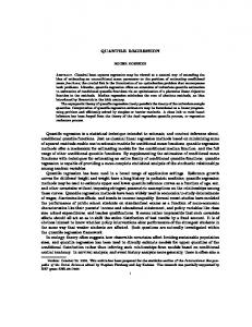
Figure 1: Plots of the exponents limd→∞ α(r, βES (d, α, θ), θ, ζ) from Theorem 4 (thick curve) and [7, Cor. 4.12] (thin curve) versus the dimension d, if the regularizing parameter λ = λn is chosen in an optimal manner for the nonparametric setup, i.e. λn = n−(2α+d)/(2α(2−θ)+d) with α = 1. We set θ = 0.5 and ζ = 1.

15

0.4 0.0

400

600

800

1000

0

200

400

600

d

d

r=0.25

r=0.5

800

1000

800

1000

0.4 0.2 0.0

0.0

0.2

exponent

0.4

0.6

200

0.6

0

exponent

0.2

exponent

0.4 0.2 0.0

exponent

0.6

r=0.125

0.6

r=0.05

0

200

400

600

800

1000

0

d

200

400

600 d

Figure 2: Similar to Figure 1, but for α = 10.

16

θ ∈ [0, 1] ζ ∈ (0, 2) >0 1 1 1/2 0 ∈ [0, 1]

fixed 1 3/2 1 fixed →2

limd→∞ αES (d, α) limd→∞ α(r, βES (d, α, θ), θ, ζ) from [7, Cor. 4.12] from Thm. 4 0 positive 0 min{r, 1/3} 0 min{r, 1/7} 0 min{r, 1/7} 0 0 0 0

Table 1: The table lists the limits of the exponents limd→∞ αES (d, α) from [7, Cor. 4.12] and limd→∞ α(r, βES (d, α, θ), θ, ζ) from Theorem 4, respectively, if the regularizing parameter λ = λn is chosen in an optimal manner for the nonparametric setup, i.e. λn = n−βES (d,α,θ) , with βES (d, α, θ) → 1 for d → ∞ and α ∈ [1, ∞). Recall that r ∈ (0, 12 ].

of SVMs for τ -quantile regression, when a single Gaussian RBF-kernel on X = Rd is used, is then of order c2 n−αES (d,α,θ) , where αES (d, α, θ) =

2α , 2α(2 − θ) + d

where c2 > 0 is a constant independent of n. If α, θ, and p are chosen such 2α+d that 2α(2−θ)+d = 4(p+1) is fulfilled with d ∈ N, we can make a fair comparison 3(p+2) between the learning rates given by [7, Cor. 4.9] and by Theorem 3, respectively. Obviously, the learning rate given in Theorem 3 favourably compares to the one given by [7, Cor. 4.9] for high dimensions d, if the assumption of an additive model is satisfied, because the exponent α(p) = 2(p+1) in The3(p+2) orem 3 is positive and independent of d ∈ N, whereas αES (d, α, θ) → 0, if d → ∞. Summarizing, the following conclusion seems to be fair. If an additive model is valid and the dimension d of X = Rd is high, then it makes sense to use an additive kernel, because (i) from a theoretical point of view: faster rate of convergence, (ii) from the big data point of view: the same accuracy of estimating the risk can in principle be achieved already with much smaller data sets, (iii) from an applied point of view: increased interpretability and flexibility.

17

r 0.5

θ 1

0.5

0.5

0.5

0.1

0.25

1

0.25

0.5

0.25

0.1

0.1

1

0.1

0.5

0.1

0.1

ζ limd→∞ α(r, βES (d, α, θ), θ, ζ) 0.1 0.5 1 0.333 1.9 0.026 0.1 0.311 1 0.143 1.9 0.013 0.1 0.05 1 0.026 1.9 0.003 0.1 0.25 1 0.25 1.9 0.026 0.1 0.25 1 0.143 1.9 0.013 0.1 0.05 1 0.026 1.9 0.003 0.1 0.1 1 0.1 1.9 0.026 0.1 0.1 1 0.1 1.9 0.013 0.1 0.05 1 0.026 1.9 0.003

Table 2: The table lists the limits of the exponents limd→∞ α(r, βES (d, α, θ), θ, ζ) from Theorem 4, if the regularizing parameter λ is chosen in optimal manner for the nonparametric setup, i.e. λ = n−(2α+d)/(2α(2−θ)+d) with α ∈ [1, ∞) and θ ∈ [0, 1], see [7, Cor. 4.12].

18

4

Proofs

This section contains all the proofs of this paper. As some of the results may be interesting in their own, we treat the topics estimation of the approximation error, the proof of the somewhat surprising assertion in Example 1, sample error estimates, and the proofs of our learning rates from Section 2 in different subsections.

4.1

Estimating the approximation error

To carry out our analysis, we need an error decomposition framework. Lemma 1. There holds RL∗ ,P (fL,Dn ,λ ) − R∗L∗ ,P,F + λkfL,Dn ,λ k2H ≤ S + D(λ),

(4.1)

where the terms are defined as S = {RL∗ ,P (fL,Dn ,λ ) − RL∗ ,Dn (fL,Dn ,λ )} + {RL∗ ,Dn (fL,P,λ ) − RL∗ ,P (fL,P,λ )} , D(λ) = RL∗ ,P (fL,P,λ ) − R∗L∗ ,P,F + λkfL,P,λ k2H .

(4.2) (4.3)

Proof. We compare the risk with the empirical risk and write RL∗ ,P (fL,Dn ,λ ) as {RL∗ ,P (fL,Dn ,λ ) − RL∗ ,Dn (fL,Dn ,λ )} + RL∗ ,Dn (fL,Dn ,λ ). Then we add and subtract a term involving the function fL,P,λ to find RL∗ ,P (fL,Dn ,λ ) − R∗L∗ ,P,F + λkfL,Dn ,λ k2H = {RL∗ ,P (fL,Dn ,λ ) − RL∗ ,Dn (fL,Dn ,λ )} 

+ RL∗ ,Dn (fL,Dn ,λ ) + λkfL,Dn ,λ k2H − RL∗ ,Dn (fL,P,λ ) + λkfL,P,λ k2H + {RL∗ ,Dn (fL,P,λ ) − RL∗ ,P (fL,P,λ )}  + RL∗ ,P (fL,P,λ ) − R∗L∗ ,P,F + λkfL,P,λ k2H . But (RL∗ ,Dn (fL,Dn ,λ ) + λkfL,Dn ,λ k2H ) − (RL∗ ,Dn (fL,P,λ ) + λkfL,P,λ k2H ) ≤ 0 by the definition of fL,Dn ,λ . Then the desired statement is proved. In the error decomposition (4.1), the first term S is called sample error and will be dealt with later on. The second term D(λ) is the approximation error which can be stated equivalently by Definition 1. In this section we estimate the approximation error based on Assumption 1. Our estimation is based on the following lemma which is proved by the same method as that in [25]. Recall that the integral operator Lkj is a positive operator on L2 (PXj ), hence Lkj + λI is invertible. 19

Lemma 2. Let j ∈ {1, . . . , s} and 0 < r ≤ 21 . Assume fj∗ = Lrkj (gj∗ ) for some gj∗ ∈ L2 (PXj ). Define an intermediate function fj,λ on Xj by fj,λ = (Lkj + λI)−1 Lkj (fj∗ ).

(4.4)

Then we have kfj,λ − fj∗ k2L2 (PX ) + λkfj,λ k2kj ≤ λ2r kgj∗ k2L2 (PX ) .

(4.5)

j

j

Proof. If {(λi , ψi )}i≥1 are √ the normalized eigenpairs of the integral operator Lkj , then the system in Hj . P { λi ψi : λi > 0} is orthogonal ∗ ∗ 2 k d ψ with k{d }k = kg Write gj∗ = i ` j L2 (PXj ) < ∞. Then fj = i≥1 i i P r i≥1 λi di ψi and fj,λ − fj∗ = Lkj + λI


−1

Lkj (fj∗ ) − fj∗ = −

X i≥1

λ λr di ψi . λi + λ i

Hence kfj,λ −fj∗ k2L2 (PX ) j

=

X i≥1

λ λr di λi + λ i

2

2r

=λ

X i≥1

λ λi + λ

2(1−r) 

λi λi + λ

2r

d2i .

Also, kfj,λ k2kj

2

2

X λ 21 +r p

X λ X λ1+2r



i i i r λi di ψi = di λi ψi = d2 . =



λi + λ λi + λ (λi + λ)2 i i≥1

kj

i≥1

kj

i≥1

Therefore, we have kfj,λ − fj∗ k2L2 (PX ) + λkfj,λ k2kj j ( 2(1−r)  2r  1−2r  1+2r ) X λ λi λ λi = λ2r + d2i λi + λ λi + λ λi + λ λi + λ i≥1   X λi λ + d2i = λ2r k{di }k2`2 = λ2r kgj∗ k2L2 (PX ) . ≤ λ2r j λ + λ λ + λ i i i≥1 This proves the desired bound.

20

4.2

Proof of Theorem 1

Proof of Theorem 1. Observe that fj,λ ∈ Hj . So f1,λ + . . . + fs,λ ∈ H and by the definition of the approximation error, we have D(λ) ≤ RL∗ ,P (f1,λ + . . . + fs,λ ) − R∗L∗ ,P,F + λkf1,λ + . . . + fs,λ k2H . But R∗L∗ ,P,F = RL∗ ,P (fF∗ ,P ) = RL∗ ,P (f1∗ + . . . + fs∗ ) according to Assumption 1. Using the inequality in (1.5), we obtain D(λ) ≤ RL∗ ,P (f1,λ + . . . + fs,λ ) − RL∗ ,P (f1∗ + . . . + fs∗ ) + λ

s X

kfj,λ k2Hj .

j=1

Applying the Lipschitz property (1.1), the excess risk term can be estimated as RL∗ ,P (f1,λ + . . . + fs,λ ) − RL∗ ,P (f1∗ + . . . + fs∗ ) Z = L∗ (x, y, f1,λ (x1 ) + . . . + fs,λ (xs )) dP (x, y) ZZ − L∗ (x, y, f1∗ (x1 ) + . . . + fs∗ (xs )) dP (x, y) Z

Z ≤ Z

s s X X |L|1 fj,λ (xj ) − fj∗ (xj ) dP (x, y) j=1

≤ |L|1

s Z X j=1

But Z Xj

j=1

fj,λ (xj ) − fj∗ (xj ) dPX (xj ) . j

Xj

fj,λ (xj ) − fj∗ (xj ) dPX (xj ) = kfj,λ − fj∗ kL1 (P ) ≤ kfj,λ − fj∗ kL2 (P ) . j Xj Xj

The bound (4.5) implies the following two inequalities kfj,λ − fj∗ k2L2 (PX ) ≤ λ2r kgj∗ k2L2 (PX j

j

)

(4.6)

and λkfj,λ k2kj ≤ λ2r kgj∗ k2L2 (PX ) . j

Taking square roots on both sides in (4.6) yields D(λ) ≤

s  X

 |L|1 kfj,λ − fj∗ kL2 (PXj ) + λkfj,λ k2Hj .

j=1

21

(4.7)

This together with (4.7) and Lemma 2 gives s n o X 2r ∗ 2 r ∗ D(λ) ≤ |L|1 λ kgj kL2 (PXj ) + λ kgj kL2 (PX ) j

j=1

and completes the proof of the statement.

4.3

Proof of the assertion in Example 1

Proof of Example 1. The function f can be written as f = f1 + 0 where f1 is a function on X1 given by f1 (x1 , x01 ) = k1 (x1 , 0) ∈ H1 . So f ∈ H. Now we prove (1.10). Assume to the contrary that f ∈ HkΠ . We apply a characterization of the RKHS HkΠ given in [20, Thm. 1] as   ∞ ∞   2 2 X X X kxk `! wα , (4.8) < ∞ wα xα : kf k2K = HkΠ = f = e− σ2 2 )` `   (2/σ C α `=0 |α|=0

|α|=`

where kxk2 = |x1 |2 + |x2 |2 and Cα` = α1`!!α2 ! for α = (α1 , α2 ) ∈ Z2+ . Since f ∈ HkΠ , we have   ∞ |x |2 +|x |2 X |x1 |2 − 1 2 2 σ f (x1 , x2 ) = exp − 2 =e wα xα σ |α|=0

where the coefficient sequence {wα : α ∈ Z2+ } satisfies kf k2K

=

∞ X `=0

X w2 `! α < ∞. (2/σ 2 )` Cα` |α|=`

It follows that  exp Hence

|x2 |2 σ2 

wα =



 m ∞ ∞ X X 1 |x2 |2 = = wα xα . 2 m! σ m=0

1 , m!σ 2m

0,

|α|=0

if α = (0, 2m) with m ∈ Z+ , otherwise,

and kf k2K

 2 X ∞ ∞ ∞ 2 X X (2m)! w(0,2m) (2m)! 1 (2m)! = = = . 2m 2 2m 2 2m 2m 2m (2/σ ) C(0,2m) m=0 (2/σ ) m!σ 2 (m!)2 m=0 m=0 22

Finally we apply the Stirling’s approximation:  m m  m m √ e √ 2πm ≤ m! ≤ √ 2πm , π π 2π and find kf k2K

∞ X

∞ X (2m)! = ≥ 22m (m!)2 m=0 m=0

p
2m √ ∞ X 2π(2m) 2m 2 π π √ = ∞.  √
m 2 = 2 m e e m 2m √ m=0 2 2πm π 2π

This is a contradiction. Therefore, f 6∈ HkΠ . This proves the conclusion in Example 1.

4.4

Sample error estimates

In this subsection we bound the sample error S defined by (4.2) by Assumption 3. It can first be decomposed in two terms: S = S1 + S2 ,

(4.9)

where RL∗ ,P (fL,Dn ,λ ) − RL∗ ,P (fF∗ ,P )  − RL∗ ,Dn (fL,Dn ,λ ) − RL∗ ,Dn (fF∗ ,P ) ,  = RL∗ ,Dn (fL,P,λ ) − RL∗ ,Dn (fF∗ ,P )  − RL∗ ,P (fL,P,λ ) − RL∗ ,P (fF∗ ,P ) .

S1 = S2



(4.10) (4.11)

The second term S2 can be bounded easily by the Bernstein inequality. Lemma 3. Under Assumptions 1 and 3, for any 0 < λ ≤ 1 and 0 < δ < 1, with confidence 1 − 2δ , we have ( r−1 r−1 θ(r+1) ) 2 λ 2 λ 2 + 4 0 √ S2 ≤ C1 log max , , (4.12) δ n n where C10 is a constant independent of δ, n or λ and given explicitly in the proof, see (4.13). Proof. Consider the random variable ξ on (Z, B(Z)) defined by ξ(x, y) = L∗ (x, y, fL,P,λ (x)) − L∗ (x, y, fF∗ ,P (x)),

23

z = (x, y) ∈ Z.

Here P B(Z) denotes the p Recall our notation for the constant p Borel-σ-algebra. κ := sj=1 supxj ∈Xj kj (xj , xj ) ≥ kkk∞ . By Assumption 1 and Assumption 3, kfF∗ ,P kL∞ (PX ) < ∞ and by Theorem 1, p p r−1 kfL,P,λ kL∞ (PX ) ≤ κkfL,P,λ kH ≤ κ D(λ)/λ ≤ κ Cr λ 2 < ∞. This in connection with the Lipschitz condition (1.1) for L tells us that the random variable ξ is bounded by   p r−1 Bλ := |L|1 kfF∗ ,P kL∞ (PX ) + κ Cr λ 2 . By Assumption 3, we also know that its variance σ 2 (ξ) can be bounded as Z

2

σ (ξ) ≤

(ξ(x, y))2 dP (x, y)

Z


2−θ  θ ≤ cθ 1 + kfL,P,λ kL∞ (PX ) RL∗ ,P (fL,P,λ ) − RL∗ ,P (fF∗ ,P )    p 2−θ p θ(r+1) r−1 2−θ Crθ λr−1+ 2 . {Cr λr }θ ≤ cθ 1 + κ Cr ≤ cθ 1 + κ C r λ 2 Now we apply the one-sided Bernstein inequality to ξ which asserts that, for all  > 0,  X    n 1 n2
. Prob ξ(zi ) − E(ξ) >  ≤ exp − n i=1 2 σ 2 (ξ) + 31 Bλ  Solving the quadratic equation 2 n2
= log 1 δ 2 σ 2 (ξ) + 3 Bλ  for  > 0, we see that with confidence 1 − 2δ , we have q
1 2 1 2 2 n X B log + B log + 2nσ 2 (ξ) log 2δ λ λ 1 3 δ 3 δ ξ(zi ) − E(ξ) ≤ n i=1 n s ( r−1 r−1 θ(r+1) ) 2 log 2δ 2 2Bλ log 2δ 2 λ 2 λ 2 + 4 √ ≤ + σ (ξ) ≤ C10 log max , , 3n n δ n n where C10 is the constant given by  p  √  p 1− θ2 θ C10 = |L|1 kfF∗ ,P kL∞ (PX ) + κ Cr + 2cθ 1 + κ Cr Cr2 . But

1 n

Pn

i=1

ξ(zi ) − E(ξ) = S2 . So our conclusion follows. 24

(4.13)

The term S1 involves the function fL,Dn ,λ which varies with the sample. Hence we need a concentration inequality to bound this term. We shall do so by applying the following concentration inequality [41] to the function set  G = L∗ (x, y, f (x)) − L∗ (x, y, fF∗ ,P (x)) : f ∈ H with kf kH ≤ R (4.14) parameterized by the radius R involving the `2 -empirical covering numbers of the function set. Proposition 1. [41, Prop. 6] Let G be a set of measurable functions on Z, and B, c > 0, θ ∈ [0, 1] be constants such that each function f ∈ G satisfies kf k∞ ≤ B and E(f 2 ) ≤ c(Ef )θ . If for some a > 0 and p ∈ (0, 2), sup sup log N2,z (G, ) ≤ a−p ,

∀ > 0,

`∈N z∈Z `

then there exists a constant c0p depending only on p such that for any t > 0, with probability at least 1 − e−t , there holds n

Ef − where

 ct 1/(2−θ) 18Bt 1 1X , f (zi ) ≤ η 1−θ (Ef )θ + c0p η + 2 + n i=1 2 n n

∀f ∈ G,

  2 2  a  4−2θ+pθ  a  2+p 2−p 2−p 4−2θ+pθ 2+p , B η := max c . n n

Lemma 4. Under Assumptions 2 and 3, for any R ≥ 1, 0 < λ ≤ 1 and 0 < δ < 1, with confidence 1 − 2δ , we have   RL∗ ,P (f ) − RL∗ ,P (fF∗ ,P ) − RL∗ ,Dn (f ) − RL∗ ,Dn (fF∗ ,P )
θ 2(1−θ) ≤ C20 R1−θ n− 4−2θ+ζθ RL∗ ,P (f ) − RL∗ ,P (fF∗ ,P ) 2 2 ∀kf kH ≤ R, (4.15) +C200 log Rn− 4−2θ+ζθ , δ where C20 , C200 are constants independent of R, δ, n or λ and given explicitly in the proof. In particular, C20 = 21 when θ = 1. Proof. Consider the function set G defined by (4.14). Each function takes the form g(x, y) = L∗ (x, y, f (x)) − L∗ (x, y, fF∗ ,P (x)) with kf kH ≤ R. It satisfies
kgk∞ ≤ |L|1 kf − fF∗ ,P k∞ ≤ |L|1 κ + kfF∗ ,P kL∞ (PX ) R =: B and by Assumption 3 and the condition R ≥ 1, E(g 2 ) ≤ (1 + κ)2−θ cθ R2−θ (Eg)θ . 25

Moreover, the Lipschitz property (1.1) and Lemma 2 imply that for any  > 0 there holds    ζ  s|L|1 R sup sup log N2,z (G, ) ≤ log N {f ∈ H : kf kH ≤ R}, ≤ scζ . |L|1  `∈N z∈Z ` Thus all the conditions of Proposition 1 are satisfied with p = ζ and we see that with confidence at least 1 − 2δ , there holds n

 c log(2/δ) 1/(2−θ) 1X 1 1−θ θ 0 Eg − g(zi ) ≤ η (Eg) + cζ η + 2 n i=1 2 n +

18B log(2/δ) , n

∀g ∈ G,

(4.16)

where c = (1 + κ)2−θ cθ R2−θ , a = scζ (s|L|1 R)ζ and   2 2  a  4−2θ+ζθ  a  2+ζ 2−ζ 2−ζ 4−2θ+ζθ 2+ζ η = max c , B . n n But Eg = RL∗ ,P (f ) − RL∗ ,P (fF∗ ,P ) and

n

1X g(zi ) = RL∗ ,Dn (f ) − RL∗ ,Dn (fF∗ ,P ). n i=1 Notice from the inequality 4 − 2θ + ζθ ≥ 2 + ζ that 2

η ≤ C30 Rn− 4−2θ+ζθ , where C30 is the constant given by
2 2−ζ C30 : = ((1 + κ)2−θ cθ ) 4−2θ+ζθ scζ (s|L|1 )ζ 4−2θ+ζθ

2−ζ
2 + |L|1 κ + kfF∗ ,P kL∞ (PX ) 2+ζ scζ (s|L|1 )ζ 2+ζ . Then our desired bound holds true with the constants given by  
1 0 1−θ 0 0 00 1/(2−θ) ∗ C2 = max (C ) , cζ C3 , 2(1 + κ)(cθ ) + 18|L|1 κ + kfF ,P kL∞ (PX ) 2 3 and C20

 =

C200 , if 0 ≤ θ < 1, 1 , if θ = 1. 2

Here the case θ = 1 can be seen directly from (4.16). This completes the proof. 26

Combining all the above results yields the following error bounds. For R ≥ 1, we denote a sample set W(R) = {z ∈ Z n : kfL,Dn ,λ kH ≤ R} .

(4.17)

Proposition 2. Under Assumptions 1 to 3, let R ≥ 1, 0 < λ ≤ 1 and 0 < δ < 1. Then there exists a subset VR of Z n with probability at most δ such that RL∗ ,P (fL,Dn ,λ ) − R∗L∗ ,P,F + λkfL,Dn ,λ k2H
θ 2(1−θ) ≤ C20 R1−θ n− 4−2θ+ζθ RL∗ ,P (fL,Dn ,λ ) − RL∗ ,P (fF∗ ,P ) ( r−1 r−1 θ(r+1) ) 2 λ 2 λ 2 + 4 √ +C10 log max , δ n n 2 2 +C200 log Rn− 4−2θ+ζθ + Cr λr , δ

∀z ∈ W(R) \ VR .

(4.18)

To apply the above analysis we need a radius R which bounds the norm of the function fL,Dn ,λ . Lemma 5. If L(x, y, 0) is bounded by a constant |L|0 almost surely, then we have almost surely p kfL,Dn ,λ kH ≤ |L|0 /λ. Proof. By the definition of the function fL,Dn ,λ , we have RL∗ ,Dn (fL,Dn ,λ ) + λkfL,Dn ,λ k2H ≤ RL∗ ,Dn (0) + λk0k2H = 0. Hence we have almost surely n

λkfL,Dn ,λ k2H

1X ≤ −RL∗ ,Dn (fL,Dn ,λ ) ≤ L(xi , yi , 0) ≤ |L|0 . n i=1

Then our desired bound follows. p Applying Proposition 2 to R = |L|0 /λ gives a learning rate. But we can do better by an iteration technique. However, we will first give the proof of Theorem 2.

27

4.5

Proofs of the main results in Section 2

Proof of Theorem 2. By the definition of the `2 -empirical covering number, for every j ∈ {1, . . . , s} and x(j) ∈ (Xj )n , there exists a set of functions
(j) {fi : i = 1, . . . , N (j) } with N (j) = N {f ∈ Hj : kf kHj ≤ 1},  such that for every f (j) ∈ Hj with kf (j) kHj ≤ 1 we can find some ij ∈ {1, . . . , N (j) } (j) satisfying d2,x(j) (f (j) , fij ) ≤ . Now every function f ∈ H with kf kH ≤ 1 can be written as f = f (1) + . . . + f (s)with kf (j) kH ≤ 1. Also, every x = (x` )n`=1 ∈ (X )n can be expressed j (1)

(s)

as x` = x` , . . . , x` (1)

(j)

with x(j) = (x` )n`=1 ∈ (Xj )n . By taking the function

(s)

fi1 ,...,is = fi1 + . . . + fis , we see that )1/2 ( n
2 1X f (x` ) − fi1 ,...,is (x` ) d2,x (f, fi1 ,...,is ) = n `=1 n  n1 X  (1) (s) = f (1) (x` ) + . . . + f (s) (x` ) n `=1  2 o1/2  (1) (1) (s) (s) − fi1 (x` ) + . . . + fis (x` ) ≤ =

s n X n  X 1 j=1 s X

n

2 o1/2 (j) (j) (j) f (j) (x` ) − fij (x` )

`=1

  (j) d2,x(j) f (j) , fij ≤ s.

j=1

The number of functions of the form fi1 ,...,is is Πsj=1 N (j) . Therefore, log N ({f ∈ H : kf kH ≤ 1}, s) ≤

s X


log N {f ∈ Hj : kf kHj ≤ 1}, 

j=1

 ζ 1 . ≤ scζ  Then our desired statement follows by scaling R to 1. We are now in a position to prove our main results stated in Section 2. Theorem 4 is proved by applying Proposition 2 iteratively. The iteration technique for analyzing regularization schemes has been well developed in the literature [29, 41, 12, 13]. p Proof of Theorem 4. Take R[0] = max{ |L|0 , 1} √1λ . Lemma 5 tells us that W(R[0] ) = Z n . We apply an iteration technique with a sequence of radii {R[`] ≥ 1}`∈N to be defined below. 28

Apply Proposition 2 to R = R[`] , and when 0 ≤ θ < 1, apply the elementary inequality 1 1 1 ∗ 1 + ∗ = 1 with q, q ∗ > 1 =⇒ a · b ≤ aq + ∗ bq , q q q q with q = 1θ , q ∗ =

1 1−θ

∀a, b ≥ 0

and

a = 2−θ RL∗ ,P (fL,Dn ,λ ) − RL∗ ,P (fF∗ ,P )


θ

2(1−θ)

,

b = 2θ C20 R1−θ n− 4−2θ+ζθ .

We know that there exists a subset VR[`] of Z n with measure at most δ such that RL∗ ,P (fL,Dn ,λ ) − R∗L∗ ,P,F + λkfL,Dn ,λ k2H 1 ≤ RL∗ ,P (fL,Dn ,λ ) − RL∗ ,P (fF∗ ,P ) 2
1 2 + 2θ C20 1−θ R[`] n− 4−2θ+ζθ ( r−1 r−1 θ(r+1) ) λ 2 λ 2 + 4 2 √ , +C10 log max δ n n 2 2 +C200 log R[`] n− 4−2θ+ζθ + Cr λr , δ

∀z ∈ W(R[`] ) \ VR[`] .

It follows that when λ = n−β for some β > 0, we have  RL∗ ,P (fL,Dn ,λ )−R∗L∗ ,P,F +λkfL,Dn ,λ k2H ≤ max an,δ R[`] , bn,δ , ∀z ∈ W(R[`] )\VR[`] , (4.19) where o n
1 2 2 00 θ 0 1−θ + 4C2 log n− 4−2θ+ζθ an,δ := 4 2 C2 δ and 2 0 bn,δ := {4C10 + 4Cr } log n−α δ with     1 θ(1 + r) 1 − r 0 α := min +β − , rβ . 2 4 2 Thus we have n β√ o √ βp kfL,Dn ,λ kH ≤ max n 2 an,δ R[`] , n 2 bn,δ ,

∀z ∈ W(R[`] ) \ VR[`] .

Hence W(R[`] ) ⊆ W(R[`+1] ) ∪ VR[`] , 29

(4.20)

after we define the sequence of radii {R[`] ≥ 1}`∈N by n β√ o √ βp R[`+1] = max n 2 an,δ R[`] , n 2 bn,δ , 1 .

(4.21)

For any positive integer J ∈ N, we have
Z m = W(R[0] ) ⊆ W(R) ∪ VR[0] ⊆ . . . ⊆ W(R[J] ) ∪ ∪J−1 `=0 VR[`] , which tells us that the set W(R[J] ) has measure at least 1 − Jδ. We also see iteratively from the definition (4.21) that n β√ o √ βp R[J] ≤ max n 2 an,δ R[J−1] , n 2 bn,δ , 1 ≤ . . . 1 n β √ 1+ 21 +...+ J−1
1 βp 2 R[0] 2J , n 2 bn,δ , 1, . . . , ≤ max n 2 an,δ 1 1 o  β√ 1+ 12 +...+ J−1  n βp o J−1 2 2 2 2 n an,δ max n bn,δ , 1 n o p
1 2 00 θ 0 1−θ 00 0 ≤ 4 2 C2 + 4C2 + 4C1 + 4Cr + 1 max{ |L|0 , 1} log nα , δ where α

00

(

 1 β α0 β β − − , + J+1 , = max 2 − J−1 2 2 4 − 2θ + ζθ 2 2 2     1 β 1 β α0 − − , ..., 2 4 − 2θ + ζθ 2 2 2    )  β 1 1 β α0 1 2 − J−1 − + J−1 − 2 2 4 − 2θ + ζθ 2 2 2   2 β α0 1 ≤ max β − , − + J 4 − 2θ + ζθ 2 2 2 ( ) 2 (1 − r)β (1 − r)β β(1 + r)(1 − 2θ ) − 1 1 = max β − , , + + J. 4 − 2θ + ζθ 2 2 4 2 1



Denote (

2 (1 − r)β (1 − r)β β(1 + r)(1 − 2θ ) − 1 α000 = max β − , , + 4 − 2θ + ζθ 2 2 4 and the constant n o p
1 θ 0 1−θ 00 0 C3 = 4 2 C2 + 4C2 + 4C1 + 4Cr max{ |L|0 , 1}. 30

)

Choose J to be the smallest positive integer greater than or equal to log2 1 . Then 21J ≤  and 2 000 R[J] ≤ C3 log nα + . δ Applying (4.19) to ` = J, we know that for every z ∈ W(R[J] ) \ VR[J] , there holds  RL∗ ,P (fL,Dn ,λ ) − R∗L∗ ,P,F ≤ max an,δ R[J] , bn,δ 2  n  o
1 2 000 2 θ 0 1−θ 0 00 ≤ C3 4 2 C2 + 4C2 + {4C1 + 4Cr } log n−min{ 4−2θ+ζθ −α , δ Since the set W(R[J] ) has measure at least 1 − Jδ while the set VR[J] has measure at most δ, we know that with confidence at least 1 − (J + 1)δ, RL∗ ,P (fL,Dn ,λ ) − where

 α = min

and Scaling Jδ Theorem 4 It only Theorem 3

R∗L∗ ,P,F

 2 2 e log ≤C m−α , δ

2 − α000 , α0 4 − 2θ + ζθ



 n o 
1 e = C3 4 2θ C20 1−θ + 4C200 + {4C10 + 4Cr } . C to δ, and expressing α explicitly, we see that the conclusion of holds true. remains to prove Theorem 3. We will do so by showing that is a special case of Theorem 4.

Proof of Theorem 3. Since P has a τ -quantile of p-average type 2 for some p p ∈ (0, ∞], we know from [27] that Assumption 3 holds true with θ = p+1 . ∞ dj Since Xj ⊂ R and kj ∈ C (Xj × Xj ), we know from [44] that Assumption 2 holds true for an arbitrarily small ζ > 0. By inserting r = 12 , β = 4(p+1) 3(p+2) p and θ = p+1 into the expression of α in Theorem 4 and choosing ζ to be sufficiently small, we know that the conclusion of Theorem 3 follows from that of Theorem 4.

References [1] F. Bach, Consistency of the Group Lasso and Multiple Kernel Learning, J. Mach. Learn. Res., 9 (2008), 1179–1225. 31

α0 }

.

[2] B.E. Boser, I. Guyon, and V. Vapnik, A training algorithm for optimal margin classifiers, in: Proceedings of the Fifth Annual ACM Workshop on Computational Learning Theory, pp. 144–152, ACM, Madison, WI, 1992. [3] A. Christmann and R. Hable, Consistency of support vector machines using additive kernels for additive models, Computational Statistics and Data Analysis 56 (2012), 854–873. [4] A. Christmann, A. Van Messem, and I. Steinwart, On consistency and robustness properties of support vector machines for heavy-tailed distributions, Statistics and Its Interface 2 (2009), 311–327. [5] C. Cortes and V. Vapnik, Support vector networks, Mach. Learn. 20 (1995), 273–297. [6] F. Cucker and D. X. Zhou, Learning Theory. An Approximation Theory Viewpoint, Cambridge University Press, Cambridge, 2007. [7] M. Eberts and I. Steinwart, Optimal regression rates for SVMs using Gaussian kernels, Electronic Journal of Statistics 7 (2013), 1–42. [8] D. Edmunds and H. Triebel, Function Spaces, Entropy Numbers, Differential Opretaors, Cambridge University Press, Cambridge, 1996. [9] T. Hastie and R. Tibshirani, Generalized additive models, Statistical Science 1 (1986), 297–318. [10] T. J. Hastie and R. J. Tibshirani, Generalized Additive Models, CRC Press, 1990. [11] T. Hofmann, B. Sch¨olkopf, and A. J. Smola, Kernel methods in machine learning, Ann. Statist. 36 (2008), 1171–1220. [12] T. Hu, Online regression with varying Gaussians and non-identical distributions, Analysis and Applications 9 (2011), 395–408. [13] T. Hu, J. Fan, Q. Wu, and D. X. Zhou, Regularization schemes for minimum error entropy principle, Analysis and Applications, to appear. [14] P. J. Huber, The behavior of maximum likelihood estimates under nonstandard conditions, Proc. 5th Berkeley Symp. 1 (1967), 221–233. [15] R. Koenker, Quantile Regression, Cambridge University Press, Cambridge. 32

[16] R. Koenker and G. Bassett, Regression Quantiles, Econometrica 46, 1978, 33–50. [17] V. Koltchinskii and M. Yuan, Sparse Recovery in Large Ensembles of Kernel Machines, In: Proceedings of COLT, (2008). [18] Y. Lin and H.H. Zhang, Component Selection and Smoothing in Multivariate Nonparametric Regression, Ann. Statist. 34 (2006), 2272-2297. [19] L. Meier, S. van de Geer, and P. B¨ uhlmann, High-dimensional Additive Modeling, Ann. Statist. 37 (2009), 3779–3821. [20] H. Q. Minh, Some properties of Gaussian reproducing kernel Hilbert spaces and their implications for function approximation and learning theory, Constr. Approx. 32 (2010), 307–338. [21] T. Poggio and F. Girosi, A theory of networks for approximation and learning, Proc. IEEE 78 (1990), 1481–1497. [22] G. Raskutti, M.J. Wainwright, and B. Yu, Minimax-Optimal Rates for Sparse Additive Models Over Kernel Classes Via Convex Programming, J. Mach. Learn. Res. 13 (2012), 389-427. [23] B. Sch¨olkopf and A. J. Smola, Learning with Kernels, MIT Press, Cambridge, M.A., 2002. [24] B. Sch¨olkopf, A.J. Smola, R.C. Williamson, and P.L. Bartlett, New support vector algorithms, Neural Comput. 12 (2000), 1207–1245. [25] S. Smale and D. X. Zhou, Shannon sampling II. Connections to learning theory, Appl. Comput. Harmonic Anal. 19 (2005), 285–302. [26] I. Steinwart and A. Christmann, Support Vector Machines, Springer, New York, 2008. [27] I. Steinwart and A. Christmann, How SVMs can estimate quantiles and the median, Advances in Neural Information Processing Systems 20 (2008), 305-312, MIT Press, Cambridge, MA. [28] I. Steinwart and A. Christmann, Estimating conditional quantiles with the help of the pinball loss, Bernoulli 17 (2011), 211–225. [29] I. Steinwart and C. Scovel, Fast rates for support vector machines using Gaussian kernels, Ann. Statist. 35 (2007), 575–607.

33

[30] C. J. Stone, Additive regression and other nonparametric models, Ann. Statist. 13 (1985), 689–705. [31] H. Sun and Q. Wu, Indefinite kernel network with dependent sampling, Anal. Appl. 11 (2013), 1350020, 15 pages. [32] J. A. K. Suykens, T. Van Gestel, J. De Brabanter, B. De Moor, and J. Vandewalle, Least Squares Support Vector Machines, World Scientific, Singapore, 2002. [33] T. Suzuki and M. Sugiyama, Fast learning rate of multiple kernel learning: trade-off between sparsity and smoothness, Ann. Statist. 41 (2013), 1381–1405. [34] I. Takeuchi, Q.V. Le, T.D. Sears, and A.J. Smola, Nonparametric quantile estimation, J. Mach. Learn. Res. 7 (2006), 1231–1264. [35] V. N. Vapnik and A. Lerner, Pattern recognition using generalized portrait method, Autom. Remote Control. 24 (1963), 774–780. [36] V. N. Vapnik, The Nature of Statistical Learning Theory, Springer, New York, 1995. [37] V. N. Vapnik, Statistical Learning Theory, John Wiley & Sons, New York, 1998. [38] G. Wahba, Support vector machines, reproducing kernel Hilbert spaces and the randomized GACV, in: Advances in Kernel Methods – Support Vector Learning (Eds. B. Sch¨olkopf, C. J. C. Burges, and A.J. Smola), MIT Press, Cambridge, MA, (1999), 69–88. [39] H. Wendland, Scattered Data Approximation, Cambridge University Press, Cambridge, 2005. [40] Q. Wu, Y. M. Ying, and D. X. Zhou, Learning rates of least square regularized regression, Found. Comput. Math. 6 (2006), 171–192. [41] Q. Wu, Y. M. Ying, and D.-X. Zhou, Multi-kernel regularized classifiers, J. Complexity 23 (2007), 108–134. [42] D. H. Xiang, Conditional quantiles with varying Gaussians, Adv. Comput. Math. 38 (2013), 723–735. [43] D. H. Xiang and D.-X. Zhou, Classification with Gaussians and Convex Loss, J. Mach. Learn. Res. 10 (2009), 1447–1468. 34

[44] D. X. Zhou, Capacity of reproducing kernel spaces in learning theory, IEEE Trans. Inform. Theory 49 (2003), 1743-1752.

Addresses: Andreas Christmann University of Bayreuth Department of Mathematics Universitaetsstr. 30 D-95447 Bayreuth Germany

Ding-Xuan Zhou City University of Hong Kong Department of Mathematics Y6524 (Yellow Zone), 6/F Academic 1 Tat Chee Avenue Kowloon Tong Hong Kong China

35