Stochastic Low-Rank Kernel Learning for Regression - arXiv

Stochastic Low-Rank Kernel Learning for Regression

Pierre Machart LIF, LSIS, CNRS, Aix-Marseille Universit´e

arXiv:1201.2416v1 [cs.LG] 11 Jan 2012

Thomas Peel LIF, LATP, CNRS, Aix-Marseille Universit´e

PIERRE . MACHART @ LIF. UNIV- MRS . FR

THOMAS . PEEL @ LIF. UNIV- MRS . FR

Sandrine Anthoine LATP, CNRS, Aix-Marseille Universit´e Liva Ralaivola LIF, CNRS, Aix-Marseille Universit´e

ANTHOINE @ CMI . UNIV- MRS . FR

LIVA . RALAIVOLA @ LIF. UNIV- MRS . FR

Herv´e Glotin LSIS, CNRS, Universit´e du Sud-Toulon-Var

Abstract We present a novel approach to learn a kernelbased regression function. It is based on the use of conical combinations of data-based parameterized kernels and on a new stochastic convex optimization procedure of which we establish convergence guarantees. The overall learning procedure has the nice properties that a) the learned conical combination is automatically designed to perform the regression task at hand and b) the updates implicated by the optimization procedure are quite inexpensive. In order to shed light on the appositeness of our learning strategy, we present empirical results from experiments conducted on various benchmark datasets.

1. Introduction Our goal is to learn a kernel-based regression function, tackling at once two problems that commonly arise with kernel methods: working with a kernel tailored to the task at hand and efficiently handling problems whose size prevents the Gram matrix from being stored in memory. Though the present work focuses on regression, the material presented here might as well apply to classification. Compared with similar methods, we introduce two novelties. Firstly, we build conical combinations of rank-1 Appearing in Proceedings of the 28 th International Conference on Machine Learning, Bellevue, WA, USA, 2011. Copyright 2011 by the author(s)/owner(s).

GLOTIN @ UNIV- TLN . FR

Nystr¨om approximations, whose weights are chosen so as to serve the regression task – this makes our approach different from (Kumar et al., 2009) and (Suykens et al., 2002), which focus on approximating the full Gram matrix with no concern for any specific learning task. Secondly, to solve the convex optimization problem entailed by our modeling choice, we provide an original stochastic optimization procedure based on (Nesterov, 2010). It has the following characteristics: i) the computations of the updates are inexpensive (thanks to the designing choice of using rank1 approximations) and ii) the convergence is guaranteed. To assess the practicality and effectiveness of our learning procedure, we conduct a few experiments on benchmark datasets, which allow us to draw positive conclusions on the relevance of our approach. The paper is organized as follows. Section 2 introduces some notation and our learning setting; in particular the optimization problem we are interested in and the rank1 parametrization of the kernel our approach builds upon. Section 3 describes our new stochastic optimization procedure, establishes guarantees of convergence and details the computations to be implemented. Section 4 discusses the hyperparameters inherent to our modeling as well as the complexity of the proposed algorithm. Section 5 reports results from numerical simulations on benchmark datasets.

2. Proposed Model Notation X is the input space, k : X ×X → R denotes the (positive) kernel function we have at hand and φ : X → H refers to the mapping φ(x) := k(x, ·) from X to the reproducing kernel Hilbert space H associated with k. Hence,

Stochastic Low-Rank Kernel Learning for Regression

k(x, x0 )=hφ(x), φ(x0 )i, with h·, ·i the inner product of H. {(xi , yi )}ni=1

n

The training set is L := ∈ (X × R) , where yi is the target value associated to xi . K = (k(xi , xj ))1≤i,j≤n ∈ Rn×n is the Gram matrix of k with respect to L. For m = 1, . . . , n, cm ∈ Rn is defined as: cm := p

1 k(xm , xm )

[k(x1 , xm ), . . . , k(xn , xm )]> .

2.2. Kernel Ridge Regression Kernel Ridge regression (KRR) is the kernelized version of the popular ridge regression (Hoerl & Kennard, 1970) method. The associated optimization problem reads: ( ) n X 2 2 min λkwk + (yi − hw, φ(xi )i) , (6) w

i=1

2.1. Data-parameterized Kernels

where λ > 0 is a regularization parameter.

˜ m is the mapping: For m = 1, . . . , n, φ˜m : X → H

Using I for the identity matrix, the following dual formulation may be considered:   1 T T α (λI + K)α . (7) max FKRR (α) := y α − α∈Rn 4λ

hφ(x), φ(xm )i φ˜m (x) := φ(xm ). k(xm , xm )

(1)

It directly follows that k˜m defined as, ∀x, x0 ∈ X , k(x, xm )k(x0 , xm ) , k˜m (x, x0 ) := hφ˜m (x), φ˜m (x0 )i = k(xm , xm ) is indeed a positive kernel. Therefore, these parameterized ˜ m )1≤m≤n of Gram makernels k˜m give rise to a family (K trices of the following form: ˜ m = (k˜m (xi , xj ))1≤i,j≤n = cm cT , K m

(2)

which can be seen as rank-1 Nystr¨om approximations of the full Gram matrix K (Drineas & Mahoney, 2005; Williams & Seeger, 2001). As studied in (Kumar et al., 2009), it is sensible to con˜ m if they are of very sider convex combinations of the K low rank. Building on this idea, we will investigate the use of a parameterized Gram matrix of the form: X ˜ ˜ m with µm ≥ 0, K(µ) = µm K (3) m∈S

where S is a set of indices corresponding to the specific rank-one approximations used. Note that since we con˜ m , which are all posisider conical combinations of the K ˜ tive semi-definite, K(µ) is positive semi-definite as well. Using (1), one can show that the kernel k˜µ , associated to ˜ our parametrized Gram matrix K(µ), is such that: k˜µ (x, x0 ) = hφ(x), φ(x0 )iA = φ(x)> Aφ(x), X φ(xm )φ(xm )> with A : = µm . k(xm , xm )

(4) (5)

m∈S

In other words, our parametrization induces a modified metric in the feature space H associated to k. On a side note, remark that when S = {1 . . . , n} (i.e. all the columns ˜ are picked) and we have uniform weights µ, then K(µ) = > KK , which is a matrix encountered when working with the so-called empirical kernel map (Sch¨olkopf et al., 1999). From now on, M denotes the size of S and m0 refers to the number of non-zero components of µ (i.e. it is the 0pseudo-norm of µ).

The solution α∗ of the concave problem (7) and the optimal solution w∗ of (6) are connected through the equality n

w∗ =

1 X ∗ α φ(xi ), 2λ i=1 i

and α∗ can be found by setting the gradient of FKRR to zero, to give α∗ = 2(I + λ1 K)−1 y.

(8)

The value of the objective function at α∗ is then: FKRR (α∗ ) = y T (I + λ1 K)−1 y,

(9)

and the resulting regression function is given by: n

1 X ∗ f (x) = α k(xi , x). 2λ i=1 i

(10)

2.3. A Convex Optimization Problem KRR may be solved by solving the linear system (I + K 3 λ )α = 2y, at a cost of O(n ) operations. This might be prohibitive for large n, even more so if the matrix I + K λ does not fit into memory. To cope with this possible prob˜ lem, we work with K(µ) (3) instead of the Gram matrix K. As we shall see, this not only makes it possible to avoid memory issues but it also allows us to set up a learning problem where both µ and a regression function are sought for at once. This is very similar to the Multiple Kernel Learning paradigm (Rakotomamonjy et al., 2008) where one learns an optimal kernel along with the target function. To set up the optimization problem we are interested in, we proceed in a way similar to (Rakotomamonjy et al., 2008). 0 ˜m For m = 1, . . . , n, define the Hilbert space H as:   kf kH˜ m 0 ˜m ˜m < ∞ . (11) H := f ∈ H µm

Stochastic Low-Rank Kernel Learning for Regression 0 ˜ = LH ˜m One can prove (Aronszajn,P 1950) that H is the ˜ ˜ RKHS associated to k = µm km . Mimicking the reasoning of (Rakotomamonjy et al., 2008), our primal optimization problem reads: ( ) n X 1 X X min λ kfm k2H˜ 0 + (yi − fm (xi ))2 , m µm {fm },µ i=1 m∈S m∈S X s.t. µm ≤ n1 , µm ≥ 0, (12) m∈S

where n1 is a parameter controlling the 1-norm of µ. As this problem is also convex in µ, using the earlier results on the KRR problem, (12) is equivalent to:   1 T T ˜ α (λI + K(µ))α min max y α − α µ≥0 4λ n o X −1 ˜ = min y T (I + λ1 K(µ)) y s.t. µm ≤ n1 . (13) µ≥0

m∈S

Finally, using the equivalence between Tikhonov and Ivanov regularization methods (Vasin, 1970), we obtain the convex and smooth optimization problem we focus on: ) ( X −1 T 1 ˜ µm . (14) min F (µ) := y (I+ K(µ)) y + ν

problem, but they may be too computationally expensive if n is very large, which is essentially due to a suboptimal exploitation of the parametrization of the problem. Instead, the optimization strategy we propose is specifically tailored ˜ to take advantage of the parametrization of K(µ). Algorithm 1 depicts our stochastic descent method, inspired by (Nesterov, 2010). At each iteration, a randomly chosen coordinate of µ is updated via a Newton step. This method has two essential features: i) using coordinate-wise updates of µ involves only partial derivatives which can be easily computed and ii) the stochastic approach ensures a reduced memory cost while still guaranteeing convergence. Algorithm 1 Stochastic Coordinate Newton Descent Input: µ0 random. repeat Choose coordinate mk uniformly at random in S. = µkm if m 6= mk and Update : µk+1 m 2

k

k

∂F (µ ) k 1 ∂ F (µ ) µk+1 (v−µkmk )2 , mk = argmin ∂µm (v−µmk )+ 2 ∂µ2 v≥0

mk

k

(18) until F (µk ) − F (µk−M ) < F (µk−M )

λ

µ≥0

m

The regression function f˜ is derived using (1), a minimizer µ∗ of the latter problem and the accompanying weight vector α∗ such that  −1 ˜ ∗) α∗ = 2 I + λ1 K(µ y, (15) (obtained adapting (8) to the case K = K(µ∗ )). We have: n n 1 X ∗˜ 1 X ∗ X ∗˜ αi k(xi , x) = f˜(x) = µm αi km (xi , x) 2λ i=1 2λ i=1 m∈S 1 X ∗ = α ˜ m k(xm , x), (16) 2λ m∈S

where

c> α ∗ ∗ α ˜m := µ∗m p m . k(xm , xm )

Notice that the Stochastic Coordinate Newton Descent (SCND) is similar to the algorithm proposed in (Nesterov, 2010), except that we replace the Lipschitz constants by the 2 F (µk ) second-order partial derivatives ∂ ∂µ . Thus, we replace 2 mk

a constant step-size gradient descent by a the Newton-step in (18), which allows us to make larger steps. We show that for the function F in (14), SCND does provably converge to a minimizer of Problem (14). First, we rewrite (18) as a Newton step and compute the partial derivatives: Proposition 1. Eq. (18) is equivalent to  (  ∂F (µk ) ∂ 2 F (µk ) k µ − / if 2 mk ∂µmk ∂µm µk+1 k + mk = 0 otherwise.

∂ 2 F (µk ) ∂µ2m

6= 0

k

(19)

(17) Proof. (19) gives the optimality conditions for (18).

3. Solving the problem We now introduce a new stochastic optimization procedure to solve (14). It implements a coordinate descent strategy with step sizes that use second-order information. 3.1. A Second-Order Stochastic Coordinate Descent Problem (14) is a constrained minimization based on the differentiable and convex objective function F . Usual convex optimization methods (such as projected gradient descent, proximal methods) may be employed to solve this

Proposition 2. The partial derivatives

∂ p F (µ) ∂µp m

are:

∂F (µ) ∂µm

˜ −1 cm )2 + ν, = −λ(y > K λ,µ

p

p−1 ˜ −1 cm )2 (c> ˜ −1 = (−1)p p!λ(y > K , m Kλ,µ cm ) λ,µ

∂ F (µ) ∂µp m

(20)

−1 ˜ −1 := (λI + K(µ)) ˜ with p ≥ 2 and K . (21) λ,µ

Proof. Easy but tedious calculations give the results. Theorem 1 (Convergence). For any sequence {mk }k , the sequence {F (µk )}k verifies:

Stochastic Low-Rank Kernel Learning for Regression

(a) ∀k, F (µk+1 ) ≤ F (µk ). k

(b) limk→∞ F (µ ) = minµ≥0 F (µ). Moreover, if there exists a minimizer µ∗ of F such that the Hessian ∇2 F (µ∗ ) is positive definite then:

and Gold , the vectors and matrices before the update and µnew , Cnew , Dnew and Gnew the updated matrices/vectors. Let also ep bethe vector whose pth coordinate is 1 while other coordinates are 0. We encounter four different cases. new Case 1: µold = 0. No update needed: p = 0 and µp

(c) µ∗ is the unique minimizer of F . The sequence {µk } converges to µ∗ : ||µk −µ∗ ||→0.

Gnew = Gold .

new Case 2: µold 6= 0. Here, Cold = Cnew and p 6= 0 and µp

∂ 3 F (µ) ∂µ3m

≤ 0 (see (20)), one Sketch of proof. (a) Using that shows that the Taylor series truncated to the second or2 (µ) 1 ∂ F (µ) der: v → F (µ) + ∂F ∂µm (v m − µm ) + 2 ∂µ2m (v m − µm )2 , is a quadratic upper-bound of F that matches F and ∇F at point µ (for any fixed m and µ). From this, the update formula (18) yields F (µk+1 ) ≤ F (µk ). (b) First note that ||µk || ≤ F (µ0 ) and extract a converging subsequence {µφ(k) }. Denote the limit by 2 ˆ F (µ) ˆ Separating the cases where ∂ ∂µ is zero or not, µ. 2 m ˆ satisfies the optimality conditions: one shows that µ ˆ v − µi ˆ ≥ 0, ∀v ≥ 0. Thus µ ˆ is a minih∇F (µ), mizer of F and we have lim F (µk ) = lim F (µφ(k) ) = ˆ = minµ≥0 F (µ). F (µ) (c) is standard in convex optimization.

−1 −1 Dnew = Dold + ∆p ep e> p,

λ,µ

|Sµ+ |.

Let = {m ∈ S|µm > 0} and m0 = kµk0 = Let C = [ci1 · · · cim0 ] be the concatenation of the cij ’s, for ij ∈ Sµ+ and D the diagonal matrix with diagonal elements µij , for ij ∈ Sµ+ . Remark that throughout the iterations the sizes of C and D may vary. Given (21) and using Woodbury formula (Theorem 2, Appendix), we have: ˜ −1 = λI + CDC > K λ,µ


−1

=

1 1 I − 2 CGC > λ λ

(22)

−1  1 . (23) G := D−1 + C > C λ Note that G is a square matrix of order m0 and that an update on µ will require an update on G. Even though updating G−1 , i.e. D−1 + λ1 C > C, is trivial, it is more efficient to directly store and update G. This is what we describe now. with

At each iteration, only one coordinate of µ is updated. Let p be the index of the updated coordinate, µold , Cold , Dold

1 1 − old . µnew µ p p

= 0. Here, Sµ+new = 6= 0 and µnew Case 3: µold p p + Sµold \ {p}. It follows that we have to remove cp from Cold to have Cnew . To get Gnew , we may consider the → 0 (that is, when previous update formula when µnew p ∆p → +∞). Note that we can use the previous formula ˜ −1 is well-defined and continuous at 0. because µp 7→ K λ,µ

3.2. Iterative Updates One may notice that the computations of the derivatives (20), as well as the computation of α∗ , depend on ˜ −1 . Moreover, the dependency in µ, for all those quanK λ,µ ˜ −1 . Thus, a special care need be taken tities, only lies in K λ,µ −1 ˜ on how K is stored and updated throughout.

where ∆p :=

Then, using Woodbury formula, we have: −1  ∆p > Gnew = G−1 + ∆ e e = Gold − g g> , p p p old 1 + ∆p gpp p p (25) with gpp the (p, p)th entry of Gold and g p its pth column.

Thus, as limµnew p →0

Sµ+

(24)

Gnew

∆p 1+∆p gpp

=

1 gpp ,

we have:   1 = Gold − gp g> , p gpp \{p}

(26)

where A\{p} denotes the matrix A from which the pth column and pth row have been removed. 6= 0. We have Cnew = = 0 and µnew Case 4: µold p  p [Cold cp . Using (23), it follows that !−1 −1 1 > > Dold + λ1 Cold Cold λ Cold cp Gnew = 1 > 1 + λ1 c> p cp λ cp Cold µnew p !−1 1 > G−1 old λ Cold cp = 1 > 1 + λ1 c> p cp λ cp Cold µnew p   A v = , v> s where, using the block-matrix inversion formula of Theorem 3 (Appendix), we have:  −1 1 1 > 1 > > s= + c c − c C G C c p old old old p µnew λ p λ2 p p s > v = − Gold Cold cp (27) λ 1 A = Gold + vv > . s

Stochastic Low-Rank Kernel Learning for Regression

Algorithm 2 SLKL: Stochastic Low-Rank Kernel Learning inputs: L := {(xi , yi )}ni=1 , ν > 0, M > 0,  > 0. outputs: µ, G and C (yield (λI + K(µ))−1 from (22)). initialization: µ(0) = 0. repeat Choose coordinate mk uniformly at random in S. Update µ(k) according to (19), by changing only the mk -th coordinate µkmk of µ(k) : •

compute the second order derivative

•

˜ −1 cm )2 (c> ˜ −1 h = λ(y > K mk Kλ,µ cmk ) ; k λ,µ if h > 0 then µ(k+1) mk

else

= max

(k) 0, µm k

(k+1)

µmk

! ;

Complete learning algorithm. Algorithm 2 depicts the full Stochastic Low-Rank Kernel Learning algorithm (SLKL), which recollects all the pieces just described.

4. Analysis Here, we discuss the relation between λ and ν and we argue that there is no need to keep both hyperparameters. In addition, we provide a short analysis on the runtime complexity of our learning procedure. 4.1. Pivotal Hyperparameter λν First recall that we are interested in the minimizer µ∗λ,ν of constrained optimization problem (14), i.e.: (28)

µ≥0

where, for the sake of clarity, we purposely show the dependence on λ and ν of the objective function Fλ,ν  X
−1 µm ˜ µ Fλ,ν (µ) = y > I + K y + λν (29) λ λ , m

˜ ∗λ,ν the weight vectors associated We may name α∗λ,ν , α ∗ with µλ,ν (see (15) and (17)). We have the following: Proposition 3. Let λ, ν, λ0 , ν 0 be strictly positive real numbers. If λν = λ0 ν 0 then 0 µ∗ 0 0 = λ µ∗ , and f˜λ,ν = f˜λ0 ,ν 0 . λ

λ,ν

As a direct consequence: ∀λ, ν ≥ 0, f˜λ,ν = f˜1,λν .

  µ∗ −1 λ0 ,ν 0 y α∗λ0 ,ν 0 = 2 I + K λ0   0 ∗ −1 µ = 2 I + K λλ λλ,ν y = α∗λ,ν , 0 ˜ ∗λ,ν /λ. The definition (16) of f˜λ,ν ˜ ∗λ0 ,ν 0 = λ0 α and, thus, α then gives f˜λ,ν = f˜λ0 ,ν 0 , which entails f˜λ,ν = f˜1,λν .

= 0.

Update G(k) and C (k) according to (24)-(27). until F (µk ) − F (µk−M ) < F (µk−M )

λ ,ν

Since the only constraint of problem (28) is the nonnegativity of the components of µ, it directly follows that λ0 µ∗λ,ν /λ is a minimizer of Fλ0 ,ν 0 (under these constraints), hence µ∗λ0 ,ν 0 = λ0 µ∗λ,ν /λ. To show f˜λ,ν = f˜λ0 ,ν 0 , it suffices to observe that, according to the way α∗λ,ν is defined (cf. (15)),

˜ −1 cm )2 − ν λ(y > K k λ,µ + h

µ∗λ,ν = argmin Fλ,ν (µ),

Proof. Suppose that we know µ∗λ,ν . Given the definition (29) of Fλ,ν and using λν = λ0 ν 0 , we have  0  Fλ,ν (µ) = Fλ0 ,ν 0 λλ µ

This proposition has two nice consequences. First, it says that the pivotal hyperparameter is actually the product λν: this is the quantity that parametrizes the learning problem (not λ or ν, seen independently). Thus, the set of regression functions, defined by the λ and ν hyperparameter space, can be described by exploring the set of vectors (µ∗1,ν )ν>0 , which only depends on a single parameter. Second, considering (µ∗1,ν )ν>0 allows us to work with the family of objective functions (F1,ν )ν>0 , which are well-conditioned numerically as the hyperparameter λ is set to 1. 4.2. Runtime Complexity and Memory Usage For the present analysis, let us assume that we pre-compute the M (randomly) selected columns c1 , . . . , cM . If a is the cost of computing a column cm , the pre-computation has a cost of O(M a) and has a memory usage of O(nM ). At each iteration, we have to compute the first and secondorder derivatives of the objective function, as well as its value and the weight vector α. Using (22), (20), (14) and (15), one can show that those operations have a complexity of O(nm0 ) if m0 is the zero-norm of µ. Besides, in addition to C, we need to store G for a memory cost of O(m20 ). Overall, if we denote the number of iterations by k, the algorithm has a memory cost of O(nM + m20 ) and a complexity of O(knm0 + M a). If memory is a critical issue, one may prefer to compute the columns cm on-the-fly and m0 columns need to be stored instead of M (this might be a substantial saving in terms of memory as can be seen in the next section). This improvement in term of memory usage implies an additive cost in the runtime complexity. In the worst case, we have

Stochastic Low-Rank Kernel Learning for Regression

5. Numerical Simulations We now present results from various numerical experiments, for which we describe the datasets and the protocol used. We study the influence of the different parameters of our learning approach on the results and compare the performance of our algorithm to that of related methods.

ν=0.01 M=1000 4.72 4.7 log(objective value)

to compute a new column c at each iteration. The resulting memory requirement scales as O(nm0 + m20 ) and the runtime complexity varies as O(k(nm0 + a)).

4.68 4.66 4.64 4.62 4.6 4.58 0

2

4 6 log(iteration)

8

10

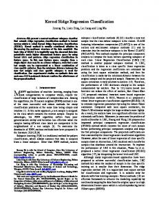
Figure 1. Evolution of the objective during the optimization process for the sinc dataset with ν = 0.01, M = 1000 (for 20 runs).

5.1. Setup

We then assess our method on two UCI datasets: Abalone (abalone) and Boston Housing (boston), using the same normalizations, Gaussian kernel parameters (σ denotes the kernel width) and data partition as in (Smola & Sch¨olkopf, 2000). The United States Postal Service (USPS) dataset is used with the same setting as in (Williams & Seeger, 2001). Finally, the Modified National Institute of Standards and Technology (MNIST) dataset is used with the same preprocessing as in (Maji & Malik, 2009). Table 1 summarizes the characteristics of all the datasets we used.

Table 1. Datasets used for the experiments.

dataset

#features

#train (n)

#test

σ2

sinc abalone boston USPS MNIST

2 10 13 256 2172

1000 3000 350 7291 60000

1000 1177 156 2007 10000

1 2.5 3.25 64 4

As displayed in Algorithm 1, at each iteration k > M , we check if F (µk )−F (µk−M ) < F (µk−M ) holds. If so, we stop the optimization process.  thus controls our stopping criterion. In the experiments, we set  = 10−4 unless otherwise stated and we set λ to 1 for all the experiments and we run simulations for various values of ν and M . In order to assess the variability incurred by the stochastic nature of our learning algorithm, we run each experiment 20 times.

350 300 final L0(mu) (mean)

First, we use a toy dataset (denoted by sinc) to better understand the role and influence of the parameters. It consists in regressing the cardinal sine of the two-norm (i.e. x 7→ sin(kxk)/kxk) of random two-dimensional points, each drawn uniformly between −5 and +5. In order to have a better idea on how the solutions may or may not over-fit the training data, we add some white Gaussian noise on the target variable of the randomly picked 1000 training points (with a 10 dB signal-to-noise ratio). The test set is made of 1000 non-noisy independent instance/target pairs.

250

nu = 1e−6 nu = 1e−4 nu = 1e−2 nu = 1

200 150 100 50 0 0

200

400

M

600

800

1000

Figure 2. Zero-norm of the optimal µ∗ as a function of M for different values of ν for the sinc dataset (averaged on 20 runs).

5.2. Influence of the parameters 5.2.1. E VOLUTION OF THE OBJECTIVE We have established (Section 3) the convergence of our optimization procedure, under mild conditions. A question that we have not tackled yet is to evaluate its convergence rate. Figure 1 plots the evolution of the objective function on the sinc dataset. We observe that the evolutions of the objective function are impressively similar among the different runs. This empirically tends to assert that it is relevant to look for theoretical results on the convergence rate. A question left for future work is the impact of the random selection of the set of columns S on the reached solution. 5.2.2. Z ERO - NORM OF µ As shown in Section 4.2, both memory usage and the complexity of the algorithm depend on m0 . Thus, it is interesting to take a closer look at how this quantity evolves. Figure 2 and 3 experimentally point out two things. On the one hand, the number of active components m0 = kµk0 remains significantly smaller than M . In other words, as long as the regularization parameter is well-chosen, we never have to store all of the cm at the same time. On the other hand, the solution µ∗ is sparse and kµ∗ k0 grows with M and diminishes with ν. A theoretical study on the dependence of µ∗ and m0 in M and ν, left for future work, would

Stochastic Low-Rank Kernel Learning for Regression ν=0.01 M=1000 400

Table 3. Number of errors and standard deviation on the test set (2007 examples) of the USPS dataset.

L0(mu)

300

200

100

0 0

1000

2000

3000 iteration

4000

5000

M

64

256

1024

Nyst

101.3 ± 22.9

34.5 ± 3.0

35.9 ± 2.0

SLKL m0

76.3 ± 9.9 61

47.6 ± 3.1 210

41.5 ± 3.9 515

6000

Figure 3. Evolution of the zero-norm of µ (m0 ) with the iterations for the sinc dataset with ν = 0.01, M = 1000 (20 runs).

be all the more interesting since sparsity is the cornerstone on which the scalability of our algorithm depends. 5.3. Comparison to other methods This section aims at giving a hint on how our method performs on regression tasks. To do so, we compare the Mean Square Error (over the test set). In addition to our Stochastic Low-Rank Kernel Learning method (SLKL), we solve the problem with the standard Kernel Ridge Regression method, using the n training data (KRRn) and using only M training data (KRRM). We also evaluate the performance of the KRR method, using the kernel obtained with uniform weights on the M rank-1 approximations selected for SLKL (Unif ). The results are displayed in Table 2, where the bold font indicates the best low-rank method (KRRM, Unif or SLKL) for each experiment. Table 2 confirms that optimizing the weight vector µ is decisive as our results dramatically outperform those of Unif. As long as M < n, our method also outperforms KRRM. The explanation probably lies in the fact that our approximations keep information about similarities between the M selected points and the n − M others. Furthermore, our method SLKL achieves comparable performances (or even better on abalone) than KRRn, while finding sparse solutions. Compared to the approach from (Smola & Sch¨olkopf, 2000), we seem to achieve lower test error on the boston dataset even for M = 128. On the abalone dataset, this method outperforms ours for every M we tried. Finally, we also compare the results we obtain on the USPS dataset with the ones obtained in (Williams & Seeger, 2001) (Nyst). As it consists in a classification task, we actually perform a regression on the labels to adapt our method, which is known to be equivalent to solving Fisher Discriminant Analysis (Duda & Hart, 1973). The performance achieved by Nyst outperforms ours. However, one may argue that the performance have a same order of magnitude and note that the Nyst approach focuses on the classification task, while ours was designed for regression.

5.4. Large-scale dataset To assess the scalability of our method, we ran experiments on the larger handwritten digits MNIST dataset, whose training set is made of 60000 examples. We used a Gaussian kernel computed over histograms of oriented gradients as in (Maji & Malik, 2009), in a “one versus all” setting. For M = 1000, we obtained classification error rates around 2% over the test set, which do not compete with state-ofthe-art results but achieve reasonable performance, considering that we use only a small part of the data (cf. the size of M ) and that our method was designed for regression. Although our method overcomes memory usage issues for such large-scale problems, it still is computationally intensive. In fact, a large number of iterations is spent picking coordinates whose associated weight remains at 0. Though those iterations do not induce any update, they do require computing the associated Gram matrix column (which is not stored as it does not weigh in the conic combination) as well as the derivatives of the objective function. The main focus of our future work is to avoid those computations, using e.g. techniques such as shrinkage (Hsieh et al., 2008).

6. Conclusion We have presented an original kernel-based learning procedure for regression. The main features of our contribution are the use of a conical combination of data-based kernels and the derivation of a stochastic convex optimization procedure, that acts coordinate-wise and makes use of second-order information. We provide theoretical convergence guarantees for this optimization procedure, we depict the behavior of our learning procedure and illustrate its effectiveness through a number of numerical experiments carried out on several benchmark datasets. The present work naturally raises several questions. Among them, we may pinpoint that of being able to establish precise rate of convergence for the stochastic optimization procedure and that of generalizing our approach to the use of several kernels. Establishing data-dependent generalization bounds taking advantage of either the one-norm constraint on µ or the size M of the kernel combination is of primary importance to us. The connection established between the one-norm hyperparameter ν and the ridge pa-

Stochastic Low-Rank Kernel Learning for Regression Table 2. Mean square error with standard deviation measured on three regression tasks. M

256

sinc 512

1000

128

0.009 ± 09

KRRn

boston 256

350

512

10.17 ± 0

abalone 1024

3000

6.91 ± 0

KRRM

0.0146 ±1e−3

0.0124 ±7e−4

0.0099 ±0

33.27 ±7.8

16.89 ±3.27

10.17 ±0

6.14 ±0.25

5.51 ±0.09

5.25 ±0

Unif

0.0124 ±1e−4

0.0124 ±3e−5

0.0124 ±0

149.7 ±5.57

147.84 ±2.24

147.72 ±0

10.04 ±0.17

9.96 ±0.06

9.99 ±0

0.0106 ±4e−4 83

0.0103 ±2e−4 108

0.0104 ±1e−4 139

20.17 ±2.3 108

13.1 ±0.87 161

11.43 ±0.06 184

5.04 ±0.08 159

4.94 ±0.03 191

4.95 ±0.004 253

SLKL m0

rameter λ, in section 4, seems interesting and may be witnessed in (Rakotomamonjy et al., 2008). Although not been mentioned so far, there might be connections between our modeling strategy and boosting/leveraging-based optimization procedures. Finally, we plan on generalizing our approach to other kernel methods, noting that rank-1 update formulas as those proposed here can possibly be exhibited even for problems with no closed-form solution. Acknowledgments This work is partially supported by the IST Program of the European Community, under the FP7 Pascal 2 Network of Excellence (ICT-216886-NOE) and by the ANR project LAMPADA (ANR-09-EMER-007).

A. Matrix Inversion Formulas Theorem 2. (Woodbury matrix inversion formula (Woodbury, 1950)) Let n and m be positive integers, A ∈ Rn×n and C ∈ Rm×m be non-singular matrices and let U ∈ Rn×m and V ∈ Rm×n be two matrices. If C −1 +V A−1 U is non-singular then so is A+U CV and: (A+U CV )−1 = A−1 −A−1 U (C −1 +V A−1 U )−1 V A−1 . Theorem 3. (Matrix inversion with added column) Given m, integer and M ∈ R(n+1)×(n+1) partitioned as:   A b M= , where A ∈ Rn×n , b ∈ Rn and c ∈ R. b> c If A is non-singular and c − b> A−1 b 6= 0, then M is nonsingular and the inverse of M is given by  −1 1 −1 > −1  − k1 A−1 b A + k A bb A M −1 = , (30) 1 − k1 b> A−1 k where k = c − b> A−1 b.

Drineas, P. and Mahoney, M. On the nystr¨om method for approximating a gram matrix for improved kernel-based learning. J. of Machine Learning Research, 6:2153–2175, Dec. 2005. Duda, Richard O. and Hart, Peter E. Pattern Classification and Scene Analysis. John Wiley and Sons, 1973. Hoerl, A. and Kennard, R. Ridge regression: applications to nonorthogonal problems. Technometrics, 12(1):69–82, 1970. Hsieh, C.-J., Chang, K.-W., Lin, C.-J., Keerthi, S. Sathiya, and Sundararajan, S. A dual coordinate descent method for largescale linear svm. In Proceedings of the 25th International Conference on Machine Learning, pp. 408–415, 2008. Kumar, S., Mohri, M., and Talwalkar, A. Ensemble nystr¨om method. In Advances in Neural Information Processing Systems 22, pp. 1060–1068, 2009. Maji, S. and Malik, J. Fast and accurate digit classification. Technical report, EECS Department, UC Berkeley, 2009. Nesterov, Y. Efficiency of coordinate descent methods on hugescale optimization problems. Core discussion papers, 2010. Rakotomamonjy, A., Bach, F., Canu, S., and Grandvalet, Y. Simplemkl. J. of Machine Learning Research, 9:2491–2521, 2008. Sch¨olkopf, B., Mika, S., Burges, C. J. C., Knirsch, P., M¨uller, K.R., R¨atsch, G., and Smola, A. J. Input space versus feature space in kernel-based methods. IEEE Transactions on Neural Networks, 10(5):1000–1017, September 1999. Smola, A. J. and Sch¨olkopf, B. Sparse greedy matrix approximation for machine learning. In International Conference on Machine Learning, pp. 911–918, 2000. Suykens, Johan A. K., Gestel, Tony Van, Brabanter, Jos De, Moor, Bart De, and Vandewalle, Joos. Least Squares Support Vector Machines, chapter 6, pp. 173–182. World Scientific, 2002. Vasin, V. V. Relationship of several variational methods for the approximate solution of ill-posed problems. Mathematical Notes, 7(3):161–166, 1970.

References

Williams, C. and Seeger, M. Using the nystr¨om method to speed up kernel machines. In Advances in Neural Information Processing Systems 13, pp. 682–688. MIT Press, 2001.

Aronszajn, N. Theory of reproducing kernels. Transactions of the American Mathematical Society, 68(3):337–404, May 1950.

Woodbury, M. A. Inverting modified matrices. Technical report, Statistical Research Group, Princeton University, 1950.