Learning Robust Color Name Models from Web Images Boris Schauerte∗ ∗ Karlsruhe Institute of Technology http:// cvhci.anthropomatik.kit.edu/ ~bschauer
Abstract We use images that have been collected using an Internet search engine to train color name models for color naming and recognition tasks. Considering color histogram bands as being words of an image and the color names as classes, we use the supervised latent Dirichlet allocation to train our model. To pre-process the training data, we use state-of-the art salient object detection and a Kullback–Leibler divergence based outlier detection. In summary, we achieve state-of-the-art performance on the eBay data set and improve the similarity between labels assigned by our model and human observers by approximately 14 %.
1
Introduction
Color is undoubtedly one of the most common and important visual attributes used in natural humanhuman communication to communicate and reference objects. There even exist psychophysical and neurophysical determinants that lead to a limited set of basic color terms across all languages from which all other color terms are considered to be derivatives (see [2, 9, 10]; see Fig. 2). Consequently, it is an important aspect of natural human-computer interaction to reliably name and recognize colors. For example, this can simplify user interfaces [7], it makes it possible to direct the attention in human-robot interaction [12], it is an important information in the context of image retrieval [1], and allows to assist visually impaired people [14]. In this contribution, we describe how we learn to name colors using a weakly labelled training data set that has been acquired using Google’s search engine. Using images from the web has several advantages such as that, for example, the training data has a high variability which leads to robust classifiers, the collection of such a data set is cheap, and it is possible to flexibly learn new color names by automatically gathering the corresponding data using Internet search engines.
Rainer Stiefelhagen∗† † Fraunhofer IOSB
[email protected]
We extend the previous work in several aspects (see [1, 13, 15, 16]): We apply state-of-the-art salient object detection to estimate the image region that is most likely described by the image’s weak label. We use Kullback– Leibler divergence ratios to remove outliers from the training data set. We propose the use of the supervised latent Dirichlet allocation in place of the probabilistic semantic latent analysis with background class.
2
Related Work
Learning object categories and attributes (e.g. [5, 6, 15, 17]) with data that has been gathered from the Internet has attracted a considerable amount of research interest throughout the last decade. Most closely related to our contribution1 is the work by Weijer et al. [15, 16] and Schauerte et al. [13] that focuses on learning to assign color names to image regions. Both authors consider the color histogram bands to be “words” of an image and the color terms as “topics”. Consequently, document analysis methods such as, e.g., the probabilistic latent semantic analysis [8] and latent Dirichlet allocation (see [3]) can be applied to learn the association between the color distribution of image regions and the corresponding color names. Weijer et al. uses a modification of the probabilistic latent semantic analysis [8] to learn the color distributions of the 11 English basic color terms [15, 16]. Schauerte et al. introduces a probabilistic HSL transformation that transforms artificial images in such a way that the characteristic of the color distribution is more similar to that of natural images [13]. Furthermore, a sampling mechanism based on the probabilistic χ 2 distance was proposed to remove outliers in the training data set [13]. Topic models determine a low dimensional representation of data under the assumption that each data point can exhibit multiple components, i.e. “topics” (see [17]). Probabilistic latent semantic analysis (PLSA) statistically analyzes the relationships between a set of 1 Please see the work by Benavente et al. [1] for an overview of computational color naming approaches.
documents and the terms they contain to produce a set of topics [8]. Weijer et al. adapted PLSA in two ways [15, 16]: First, they directly linked the topics with the class labels, effectively turning PLSA into a supervised multi-class learning approach. Second, they introduced a background class that is shared across all topics and reflects that the images often contain a foreground object on a (simple) background, see Fig. 1 and 2. However, PLSA has two main deficits: First, it is known for overfitting problems. Second, it is not a generative model of new documents, although being a generative model of the documents in the collection it is trained on. Both aspects are problematic for our application. The latent Dirichlet allocation (LDA; see [3]) is closely related to PLSA, except that it assumes that the topic distribution has a Dirichlet prior. Most importantly, LDA is a generative model for new documents. Blei et al. introduced supervised LDA (SLDA), which is able to learn the topic distributions and associate them with labels in a supervised fashion [3]. Multi-class SLDA is an extension of SLDA and was introduced by Wang et al. [17]. It combines generative and discriminative methods, and it allows to work with discrete class labels such as, e.g., color terms as in our application.
3
Learning Color Models
Similar to learning topics in bag-of-word models in text analysis, we try to learn color terms Z = {z1 , ..., zK } in a bag-of-pixel representation, i.e. a color histogram. Images and image regions D = {d1 , ..., dN } are represented by histograms whose bins are interpreted as words W = {w1 , .., wM }. Each image d is (weakly) labelled with its color term ld = t.
3.1
Salient Object Detection
To support the learning process, it is beneficial to suppress image content that is not related to the label we want to learn. To this end, Weijer et al. suppress pixels with the same color as the image border (see [16]). Alternatively, the pHSL transformation by Schauerte et al. effectively reduces the influence of the often monochromatic background by distributing it over a wide range of histogram bins [13]. Following the approach by Weijer et al. (see [16]), we first suppress pixels that have a similar color as the image border. Despite its simplicity this method works well for “artificial” images, see Fig. 1 (middle row). A background is detected, if the border color’s mean standard deviation over all image channels is below a threshold of 0.01 (RGB in [0, 1]3 ). Then, we sup-
green red yellow Figure 1. Example images (top) with their estimated foreground mask (middle) and salient object detection (bottom).
press all pixels whose distance to the mean image border color is less than 0.01 (see Fig. 1). However, the simple background suppression does not work for complex or natural images, see Fig. 1 (bottom row). Therefore, we use the salient object detection method by Cheng et al. [4] to estimate the image regions that most likely contain the object of interest. We use the saliency map that is provided by Cheng’s algorithm to weight each pixel’s entry in the histogram. This way, image regions that are likely to contain the target concept have a higher influence than regions that are unlikely to contain the target object (see Fig. 1).
3.2 Outlier Reduction We try to determine outliers in the training data set by estimating an initial word observation model P(w|z) and subsequently removing images whose distribution diverges from the initial estimate (see Fig. 2). For this purpose, it is possible to use probability distribution distances such as, e.g., the χ 2 distance (as in [13]) or the Kullback–Leibler divergence (see [11]). The Kullback– Leibler divergence DKL (PkQ) (KLD), also known as relative entropy, is a non-symmetric measure of the difference between two probability distributions P and Q. From an information theoretic perspective the KLD measures the expected number of additional bits that would be required to code samples using a code based on Q instead of P. Using the mean probabilities as initial models P0 (w|z) for the color terms, we calculate the KLD between each initial model and document zd dKLD (P0 (·|z), P(·|d)) =
P(w|d)
∑ P(w|d) ln P0 (w|z) (1) w
0
with P (w|z) =
1 ∑ P(w|d) . (2) N d∈D,l =z d
Black Grey White Red Green Blue Yellow Orange Pink Purple Brown Figure 2. Rows 1-3: Example images from the Google-512 data set [13] for each of the 11 basic English color terms (3rd row: outliers). Row 4: Example images from the eBay data set [15].
Then, we rank the images by their KLD ratios Rzd KLD Rzd KLD =
zd dKLD
0
zd minz0 6=z dKLD
.
(3)
Rzd KLD becomes smaller the better the initial model of term z describes the image, compared to the alternative terms z0 . Consequently, Rzd KLD is greater than 1, if another color term z describes the document d better. This way, we can use a pre-defined amount of documents with the lowest KLD ratios to train the final models.
3.3
Learning and Classification
In contrast to Weijer’s PLSA-bg [15], multi-class SLDA2 does not explicitly associate the latent variables with the class labels [17]. Instead, SLDA uses the topic assignments of each histogram band as latent features for classification, effectively combining aspects of generative and discriminative classification. Consequently, during training SLDA learns topics that are predictive for the class labels in combination with class coefficients for each topic. In order to being able to assign class labels, i.e. color names, to image regions, it uses softmax regression on basis of the topic assignments, the learned class coefficients, and the topic frequencies.
4
Evaluation
We use the Google-512 data set [13] to train our color term models. The data set consists of 512 images that were collected using Google’s image search 2 Due to the complexity of multi-class SLDA’s learning and inference procedure (please also consider the limited number of available pages), we decided to keep our description short and would like to refer the interested reader to the original work by Wang et al. for algorithm details (see [17] and also [3]).
for each of the eleven basic English color terms (see Fig. 2). We use the eBay data set [15] to evaluate the classification accuracy of the learned color term models. The data set consists of segmented images of 4 object classes (cars, glass & pottery, shoes, and dresses) with 10 evaluation images for each of the 11 basic color terms (see Fig. 2). The eBay data set has been applied by – most importantly – Weijer et al. [1, 15, 16] and Schauerte et al. [13] for evaluation. To measure the quality of our trained color term model, we analyze the accuracy with which we assign the correct color label to the objects in the eBay data set (see Fig. 2). To serve as a reference, we compare our results against the two state-of-the-art models: The model that was trained by Schauerte et al. using χ 2 ranking [13] and the model that was trained using PLSA-bg only by Weijer et al. [16]. The model by Weijer et al. uses the L*a*b* color space, divided into 10×20×20 histogram bins, whereas the model by Schauerte et al. uses the pHSL color space, divided into 32×8×8 bins. For both models, we assign the color term with the maximum likelihood for classification. Serving as a natural baseline, Schauerte et al. have shown that humans achieve an average accuracy of 90.64 % on the eBay data set, which is caused by the fact that colors terms have no sharp boundaries and thus there may be more than one appropriate term in certain situations. For example, in many situations a natural confusion exists between “orange” and “red”, but there typically is no confusion between “red” and “green” (color opponents). We trained our model using SLDA with 550 latent topics and 11 classes, i.e. the 11 basic English color terms, on the Google-512 data set. We use the Lab color space with 32×32×32 histogram bins. As training samples for the SLDA, we kept the 50 % of the images that lie within the 5 and 55 percentile of the ranked Kullback–Leibler divergences from the initial estimate
Method our approach χ 2 rank [13] PLSA-bg [16] Human [13]
Cars 73.63 73.63 71.82 92.73
Pott. 80.90 79.01 83.64 87.82
Shoes 91.82 92.73 92.73 90.18
Dress 90.00 88.18 86.36 91.99
Total 84.09 83.41 83.64 90.64
Dist 0.50 0.57 0.73 0.00
Table 1. Evaluation results (in %). of each term. The choice of 550 latent topics is a tradeoff (consider that 550/323 = 0.0167), because a higher number of latent topics would provide more latent features for classification while on the other hand it increases the risk of overfitting. Our classification results on the eBay data set are shown in Tab. 1. On the first sight, the total performance of the color models is not drastically different, so let us use the next two paragraphs to explicate why our approach is an improvement. First of all, our model has the best performance for the object classes dresses and cars. The overall low performance for the classes pottery and cars can be explained with difficult object surfaces that, for example, often exhibit a considerable amount of reflection. Unfortunately, the performance of our model on the pottery class is substantially lower than the performance of Weijer’s model. However, we have to consider that the pottery class is particularly hard, because it also has the highest confusion among human raters. It is important to consider the human performance on the class shoes, because here our model has the worst accuracy, but – in consequence – it is closer to the human accuracy. As has been done by Schauerte et al. [13], we assess the naturalness of our model by calculating the similarity between the labels assigned by humans and the trained models. As evaluation measure, we use the distance between the confusion matrices of the human observers and the trained model, see Tab. 1 (rightmost column). With a distance of 0.73 the model by Weijer et al. [15,16] has the worst similarity, which indicates that it has a tendency to make “unnatural” naming mistakes. The model trained with χ 2 ranking performs substantially better with a distance of 0.57 (see [13]). However, our SLDA model has an even lower distance of 0.50, a further improvement of ∼ 14 % towards assigning natural, human-like color names to real-world image data.
5
Conclusion
We described how we learn color models from image data that was collected using Google’s search engine. We use Weijer’s heuristic and Cheng’s region contrast saliency to highlight the image region that most likely contains the object of interest. Then we use the
Kullback–Leibler divergence from each image to an initial model to detect and remove images whose color distribution is likely to be dominated by a color different from the image’s label. Finally, we use the supervised latent Dirichlet allocation to train our color name model. This way, we achieve state-of-the-art performance on the eBay data set and, most importantly, are able to improve the similarity between labels assigned by our model and humans by 14 %, reducing the number of “unnatural” naming mistakes.
References [1] R. Benavente, J. Van De Weijer, M. Vanrell, et al. Color Names. In T. Gevers, A. Gijsenij, J. van de Weijer, and J.-M. Geusebroek, editors, Color in Computer Vision. Wiley, 2011. [2] B. Berlin and P. Kay. Basic color terms: their universality and evolution. University of California Press, 1969. [3] D. Blei and J. McAuliffe. Supervised topic models. In NIPS, 2007. [4] M.-M. Cheng, G.-X. Zhang, N. J. Mitra, et al. Global contrast based salient region detection. In CVPR, 2011. [5] R. Fergus, F.-F. Li, P. Perona, and A. Zisserman. Learning object categories from Google’s image search. In ICCV, 2005. [6] V. Ferrari and A. Zisserman. Learning visual attributes. In NIPS, 2007. [7] J. Heer and M. Stone. Color naming models for color selection, image editing and palette design. In CHI, 2012. [8] T. Hofmann. Probabilistic latent semantic indexing. In SIGIR, 1999. [9] D. Lindsey and A. Brown. Diversity in English color name usage. J. Vis., 8(6):578–578, 2008. [10] A. Mojsilovic. A computational model for color naming and describing color composition of images. IEEE Trans. Image Processing, 14(5):690–699, 2005. [11] Y. Rubner, C. Tomasi, and L. J. Guibas. The earth mover’s distance as a metric for image retrieval. Int. J. Comp. Vis., 40(2):99–121, 2000. [12] B. Schauerte and G. A. Fink. Focusing computational visual attention in multi-modal human-robot interaction. In ICMI, 2010. [13] B. Schauerte and G. A. Fink. Web-based learning of naturalized color models for human-machine interaction. In DICTA, 2010. [14] B. Schauerte, M. Martinez, A. Constantinescu, and R. Stiefelhagen. An assistive vision system for the blind that helps find lost things. In ICCHP, 2012. [15] J. van de Weijer, C. Schmid, and J. J. Verbeek. Learning color names from real-world images. In CVPR, 2007. [16] J. van de Weijer, C. Schmid, J. J. Verbeek, and D. Larlus. Learning color names for real-world applications. IEEE Trans. Image Processing, 18(7):1512– 1524, 2009. [17] C. Wang, D. Blei, and L. Fei-Fei. Simultaneous image classification and annotation. In CVPR, 2009.