Web-based Learning of Naturalized Color Models for Human ... - cv:hci

Web-based Learning of Naturalized Color Models for Human-Machine Interaction Boris Schauerte Robotics Research Institute TU Dortmund University 44221 Dortmund, Germany [email protected]

Abstract— In recent years, natural verbal and non-verbal human-robot interaction has attracted an increasing interest. Therefore, models for robustly detecting and describing visual attributes of objects such as, e.g., colors are of great importance. However, in order to learn robust models of visual attributes, large data sets are required. Based on the idea to overcome the shortage of annotated training data by acquiring images from the Internet, we propose a method for robustly learning natural color models. Its novel aspects with respect to prior art are: firstly, a randomized HSL transformation that reflects the slight variations and noise of colors observed in real-world imaging sensors; secondly, a probabilistic ranking and selection of the training samples, which removes a considerable amount of outliers from the training data. These two techniques allow us to estimate robust color models that better resemble the variances seen in realworld images. The advantages of the proposed method over the current state-of-the-art technique using the training data without proper transformation and selection are confirmed in experimental evaluations. In combination, for models learned with pLSA-bg and HSL, the proposed techniques reduce the amount of mislabeled objects by 19.87 % on the well-known E-Bay data set. Keywords-Web–based/Internet–based learning, natural images, color, color terms, color naming, probabilistic HSL model, human–machine/human–robot interaction

I. I NTRODUCTION An important aspect of human-human and human-robot interaction (HRI) is the goal to establish mutual agreement about the association between communicated concepts and their physical correlates in the real world (cf. [1]). Usually, such relations are established by combining deictic references in natural language with non-verbal cues, such as gestures or gaze. In this combination gaze and gesture are mainly used to communicate spatial relations, and verbal descriptions complement these by specifying attributes or categories of intended reference objects. The latter are mandatory, if non-verbal cues alone – e.g., pointing – are not sufficient to correctly identify the intended object. Consequently, multi-modal HRI systems need to be able to robustly recognize and describe object properties in order to resolve potential ambiguities.

Gernot A. Fink Dept. Computer Science TU Dortmund University 44221 Dortmund, Germany [email protected]

Models for visual attributes can in principle be learned from sample data (cf., e.g., [2]). However, classical supervised learning techniques require the training data to be correctly annotated. This requirement is especially problematic in dynamic environments considered in HRI. There, training data labelled by experts usually is available in extremely limited quantities only. In order to resolve this problem, there exist two fundamental possibilities for acquiring annotated data. Firstly, it can be generated interactively by prompting the user. Though the quality of labelled data that can be obtained in such a manner is rather high, such a process is difficult to realize, time consuming, and able to generate rather limited sample sets only. Secondly, as pioneered by Fergus et al. [3], the Internet can be used as a source of weakly labelled data by making use of publicly available search engines. This process allows relatively fast access to a huge amount of labelled data, for which, however, the annotations are not completely reliable. In this contribution we propose a method for learning robust color models based on images acquired from the Internet. The method was inspired by Weijer et al. [4], [5], who try to achieve robustness in color naming by using larger amounts of real-wold images, i.e. the ones retrieved from the Internet. However, data sets composed of images obtained via Internet search engines suffer from at least two deficiencies. First, the images are often heavily quantized as a consequence of image compression or even completely artificial (cf. Fig. 4). Consequently, color distributions learned from such data perform poorly when applied to the classification of real, noisy image data. Therefore, we propose the use of a probabilistic HSL color model in order to generate more realistic variance in the training data and, consequently, obtain color models with better generalization capabilities. Secondly, image sets retrieved for some specific object color may contain anything ranging from oversimplified images to hardly matching ones and even completely “false positives”. Training with such noisily labelled data necessarily has a negative affect on the quality of the statistical color model obtained. Therefore, we propose to perform a preselection of training images based on a simple initial model

and an estimate of the labels’ correctness derived from the χ2 distance between the initial color and background distributions. The rest of this paper is organized as follows: We briefly overview the related work in the following Section II. In Section III and IV, we present our randomized HSL color space and explain how the color terms are learned, respectively. Subsequently, in Section V, we present the relevant data sets and discuss our evaluation results. Finally, we conclude with a brief summary and outlook in Section VI. II. R ELATED W ORK Learning object categories (e.g. [3]) and visual attributes (e.g. [2], [4]–[6]) with data acquired from the Internet has attracted an increasing interest in recent years. While [6] investigates the general “visualness” of labels assigned to images, [2] and [4], [5] focus on specific attributes, i.e. texture or color, respectively. Most closely related to our contribution is the work by Weijer et al. [4], [5] that focuses on learning to assign color names to pixels and retrieve images with specific colors. Interpreting the color histogram bands as “words” of an image and the color terms as “topics”, document analysis methods can be applied in order to learn the association between images and color names. Accordingly, in [4], [5] modifications of the probabilistic latent semantic analysis [7] are used in order to learn the color histogram distributions of the 11 English basic color terms (cf. [8]–[11]). The cross-cultural concept of basic color terms states that there exist psychophysical and neurophysical determinants that lead to a limited set of basic color terms in each language of which all other colors are considered to be variants (e.g. the 11 basic color terms for English are: “black,” “white,” “red,” “green,” “yellow,” “blue,” “brown,” “orange,” “pink,” “purple,” and “gray”). When working with color information on digital computers, the choice of an appropriate color space is of utmost importance and should be tightly coupled to the goal of the application (cf. [12]). Accordingly, there exists a wide range of established color models. For example, RGB is a device-dependent additive color space, which is often transformed into the cylindrical Hue-Saturation-Lightness (HSL) or Hue-Saturation-Value (HSV) space in order to increase intuitivity and approximate perceptual color spaces (cf. [11]). Perceptual color spaces incorporate considerations how humans perceive colors. For example, L*a*b* (also known as CIELAB) tries to normalize the perceptual distance between colors and approximate perceptual uniformity (cf. [12]), i.e. the property that equal differences of colors in the color space should produce equally important color changes in human perception. Extending that approach, color appearance models (e.g. CIECAM02 (cf. [12])) additionally apply chromatic adaptation transformations (e.g. CIECAT02 in CIECAM02) that further model the influence of the viewing conditions and surround. This is also related to

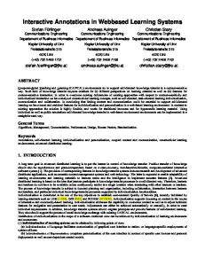
Figure 1. Images and their HS (green) and pHS (red) marginal distributions. L: image; C: hue; R: saturation (with exemplary randomization parameters ps = pb = 3). Top: artificial image shows unnatural peaks at zero hue (i.e. “red”) and saturation in the corresponding channels, which are smoothed when applying the probabilistic model. Bottom: for comparison, the smooth hue channel is only slightly affected for the natural image. However, due to the high percentage of nearly black pixels and chosen randomization parameters, the saturation distribution is notiecably influenced (please note that this is an extreme example), but without affecting the perceived visual quality.

color constancy methods which try to model the human ability to perceive the color of objects relatively constant under varying illumination conditions. In [4], [5], instead of applying color appearance or constancy methods, the huge illumination, viewing, and composition variances of images acquired from the Internet are assumed to produce robust color term models. Furthermore, the L*a*b* color space is favored for learning and naming color terms, mainly due to its perceptual properties and the better performance of the learnt model for image retrieval when compared to RGB and HSL. Interestingly, in [10] the equidistant perceptual similarity metric for Lab is critically discussed for color naming and HSL is favored. In order to model color noise and boundaries in images, probabilistic parametric models of color distributions have previously been applied in the area of color-based image segmentation (e.g. [12]–[14]). Most closely related to our probabilistic HSL model is the probabilistic HSV model in [13]. The distribution of the hue and saturation are assumed to be independent. Accordingly, the joint distribution can be modeled by a von-Mises and a Gaussian distribution while keeping the value fixed. III. P ROBABILISTIC C OLOR M ODEL A large amount of images acquired from public image search engines is synthetic, artificial, or highly processed (cf. Fig. 4). Since the color distributions of such composed images are heavily quantized or distorted, they exhibit different probability distributions compared to real-world images that are acquired with imaging sensors (cf. Fig. 1). In contrast, natural images always have slight color variations and noise, leading to a smoother distribution of colors in the image. Therefore, when training a color model on Internet image data and aiming at its application in real-world

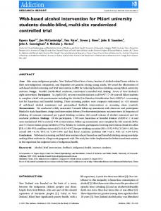
Figure 2. Example of the influence of the randomization parameters pb and ps . Left-to-right: original image, image randomized with pss = pb = 0, pss = pb = 1, and pss = pb = 4. As can be seen, increasing the parameters pb and ps improves the perceptual quality up to the point that no visual difference can be perceived.

settings, this results in a mismatch between the statistical characteristics of training and test data. Therefore, we introduce a probabilistic color model and a transformation that approaches natural color distributions for artificial images. A. Model We define our probabilistic Hue-Saturation-Lightness (pHSL) color model based on the common deterministic HSL model. Our model reflects that the measured hue and saturation get less reliable, the more the color approaches achromaticity (cf. Fig. 1). As it can be assumed that the lightness l becomes more reliable instead, we do not model it as a random variable. Consequently, we define it as equal to the deterministically determined lightness ld = l. We model the distribution of the natural hue h with a von-Mises distribution 1 κ cos(x−µ) fVM (x; µ, κ) = e , (1) 2πI0 (κ) µ=hd

where µ is set to the deterministic hue hd and I0 (κ) is the modified Bessel function of order 0. The concentration parameter κ is an inverse measure of the dispersion, i.e. κ−1 is analogous to the variance σ 2 . Similarly, the natural distribution of the saturation s is modeled using a truncated normal distribution x−µ 1 f ( ) N σ σ . (2) fT N (x; µ, σ, a, b) = b−µ a−µ µ=sd FN ( σ ) − FN ( σ ) a=0 b=1

fN is the probability density function of the standard normal distribution and FN its cumulative distribution function. The distribution is concentrated around the deterministic saturation sd = µ within the interval from a = 0 to b = 1. In this model, κ and σ control the concentration of the probability distribution of the hue and saturation, respectively, when given the observed values. In the extreme case, when κ → ∞ and σ → 0, the distributions approach a Dirac distribution and converge against the observed values. Furthermore, if κ → 0 and σ → ∞, the distributions approach the uniform distribution, which is, e.g., suitable to model the distribution of the hue for (nearly) monochrome colors.

B. Randomized HSL Transform When given an image with deterministically determined HSL values, we randomly draw the pHSL values from the distributions as defined above. Critical for this process are the choices of κ and σ, because they define the perceptual quality of the randomized image (see Fig. 2). At this point we have to consider two conflicting criteria: firstly, we do not want to change the visual perception of the randomized image compared to the original image, and, secondly, we want to maximize the entropy of the hue and saturation distributions. In this contribution, we calculate κ according to κ = (1 − s)−ps (1 − b)−pb − 1 , (3) where b = 2 min (l, 1 − l) ∈ [0, 1] is the normalization term of the chroma when calculating the saturation in the HSL model1 and serves as a lightness-dependent indicator of the colorfulness. Accordingly, the exponents ps and pb control the degree of randomization of the hue. Exploiting that the von-Mises distribution approaches a normal distribution for large concentrations κ, we can now calculate σ according to σ = κ−1/2

.

(4)

Consequently, the only parameters controlling the degree of randomization are the exponents pb and ps . They depend on the lightness and saturation, respectively, and have to be chosen depending on the desired degree of randomization, i.e. entropy, versus the expected perceptual quality of the randomized image. IV. L EARNING C OLOR T ERMS Computational color representations always need to be defined with respect to some color space. However, in order to be used for human-machine interaction, they also need to be related to a linguistic concept of color that can be communicated verbally. This accounts for the fact that “color spaces allow us to specify or describe colors in unambiguous manner, yet in everyday life we mainly identify colors by their names. Although this requires a fairly general color vocabulary and is far from being precise, identifying a color 1 1 lightness: l = (max (r, g, b) + min (r, g, b)), chroma: c 2 c max (r, g, b) − min (r, g, b), saturation: s = 2 min(l,1−l)

=

was drawn from the population represented by the other (cf. [15]). By ranking the images according to their χ2 distance ratios Rχzd2 Rχzd2 =

Figure 3. Characteristic ranked (left) and 512 (right) images.

χ2 -distance-ratio

zd Rχ 2

curves for 128

by its name is a method of communication that everyone understands” [10].

Analogue to discovering latent topics in bag-of-word models in text analysis, we try to find color terms Z = {z1 , ..., zK } in a bag-of-pixel representation, i.e. a color histogram. Accordingly, images and image regions D = {d1 , ..., dN } are represented by histograms whose bins are interpreted as words W = {w1 , .., wM }. Furthermore, each image d is weakly labelled with its topic ld = t. 1) pLSA-BG: In the probabilistic Latent Semantic Analysis (pLSA) model [7], the P probability of a word w in an image d is P (w|d) = z∈Z P (w|z)P (z|d). pLSA-bg extends this model by introducing a latent background color distribution P (w|bg), which is shared between all images. Consequently, the probability of a word w in an image d which is labeled with the latent topic z is described as a weighted mixture of the foreground distribution – i.e. the model for color z and a shared background distribution as P (w|d, ld = z) = αd P (w|ld = z) + (1 − αd )P (w|bg). The parameters of this model, namely the color-specific distributions P (w|z), the global background model P (w|bg), and the document-specific foreground probabilities αd , can be estimated using the EM algorithm as shown in [4]. 2) χ2 Ranking: As alternative to pLSA-bg and as method to calculate an initial model for the EM-algorithm of pLSA-bg, we apply a ranking procedure.PTherefore, we use the mean probabilities P 0 (w|z) = N1 d∈D,ld =z P (w|d) as initial models. Using these models, we calculate the χ2 0 distances dzd χ2 between the initial models P (·|z) and images P (·|d) 0 dzd χ2 (P (·|z), P (·|d)) =

X (P (w|d) − m)2 m

(5)

w∈W

with m=

P 0 (w|z) + P (w|d) . 2

(6)

The χ2 distances asymptotically approach the χ2 distribution and measure how unlikely it is that one distribution

0

minz0 6=z dzχ2d

,

(7)

we obtain the characteristic curves as depicted in Fig. 3. We observed these characteristic curves for multiple color models, independently of the number of considered images. By selecting the images D0 ranked along the central linear segment of the curve (cf. Fig. 3), we estimate the models according to P (w|z) =

A. Learning Color Models

dzd χ2

1 N

X

P (w|d) .

(8)

d∈D 0 ,ld =z

This selection criterion reflects that the initial model is degraded by the huge amount of background and outliers. Consequently, a considerable amount of images with a huge percentage of background is located in the head of the curve and omitting these samples, at least initially, may improve the results. Furthermore, complete outliers still differ substantially from the initial model and are located in the tail. Thus, most of the samples in the tail can be discarded. B. Assigning Color Terms In order to assign a color term z ∈ Z to an image or image region d, we first calculate the posterior probabilities P (ld = z|w) ∝ P (w|ld = z)P (ld = z) for each word w ∈ d. Using these posteriors, we assign each region to the term with the highest likelihood Y ld = arg max P (w|ld = z) , (9) t

w∈d

assuming a uniform color name prior P (ld = z). V. E VALUATION A. Data Sets For the training of our model, we used the Google image search to collect a data set of 512 images (G OOGLE -512) for each of the 11 basic color terms (see Fig. 4). As in [5], we queried for "$colorname+color". But, in contrast to the G OOGLE -250 data set in [5], we did not apply any preprocessing methods to the images. For the evaluation, we are using the E-BAY data set that is publicly available and has been applied in [4] and [5]. The data set consists of segmented images of 4 object classes (cars, glass & pottery, shoes, and dresses) with 10 evaluation images for each of the 11 basic color terms (see Fig. 4).

Black

Grey

White

Red

Green

Blue

Yellow

Orange

Pink

Purple

Brown

Figure 4. Example images from the training and evaluation data sets for each color term. Rows 1-3: 1st, 111th and 256th image of the G OOGLE -512 data set. Last row: E-BAY data set examples. Method

Space

Cars

χ2 rank pLSA-bg

HSL HSL

73.63 69.18

Randomized 92.73 87.36

88.18 87.36

79.01 83.41 77.36 81.32

χ2 rank pLSA-bg

HSL HSL

68.18 66.36

Deterministic 91.81 90.00

87.27 85.45

76.36 80.90 73.63 79.31

Reference 92.73 90.18

86.36 91.99

83.64 83.64 87.82 90.64

Weijer et al. L*a*b* 71.82 Human Brain 92.73

Shoes

Dresses

Pottery

Total

Table I P ERCENTAGE OF CORRECTLY LABELLED OBJECTS OF THE E-BAY DATA SET. T HE RANDOMIZATION ACCORDING TO THE PROBABILISTIC MODEL AS WELL AS THE χ2 RANKING SIGNIFICANTLY IMPROVE THE RECOGNITION RATE . I N COMBINATION THE PROPOSED TECHNIQUES INCREASE THE RECOGNITION RATE BY 4.1 % UP TO 83.41 %, I . E . A 19.87 % DECREASE OF MISLABELED OBJECTS . F OR COMPARISON , HUMAN OBSERVERS ASSIGN THE ANNOTATED LABEL TO 90.64 % OF THE SAMPLES .

B. Results In the following we present our results in assigning the correct color term to the objects in the E-BAY data set (see Fig. I). In order to provide comparative figures, we trained a non-probabilistic HSL model with pLSA-bg and χ2 ranking. Additionally, as a baseline, we compare our results with the pLSA-bg model presented by Weijer et al. in [4] (cf. Tab. I), which is publicly available. This model uses the L*a*b* color space, divided into 10×20×20 histogram bins. Furthermore, reflecting that borders between color terms are fuzzy (cf. [9], [10]), we performed a user study in order to assess the practically achievable recognition rate on the EBAY data set (cf. Tab. I). Therefore, we asked 5 participants to assign one of the 11 English basic color terms to each of the 440 test images in the data set. The images were displayed on a monitor upon grey background (w/o any focal, prototypic colors that could serve the annotator as orientation) in an environment with controlled illumination. Please note that we did not indicate the segmentation masks to the participants. However, this only influences the small amount of ambiguous samples (approx. 1% of the data set).

In this contribution, we refer to the following parametrization: pb = 6 and ps = 4 are used as randomization exponents of the κ-function (Eq. 1). The HSL color space is divided into 32 × 8 × 8 histogram bins. Furthermore, when χ2 ranking is applied, the images are ranked with the χ2 metric ratios (Eq. 7) and the images within the rank interval [0.275N ; 0.9N ] are selected. As it can clearly be seen in Tab. I, the randomization as well as the χ2 ranking improved the recognition rates of the learned model. The combination of probabilistic resampling and χ2 ranking improved the recognition rate by 4.1 % up to a total rate of 83.41 %. This result is comparable to the 83.64 % of the model by Weijer et al. (see Tab. I), which was learned using pLSA-bg with L*a*b as color space (see Sec. V-A). However, it has to be considered that – in contrast to the model by Weijer et al. – we did not apply any preprocessing steps such as, e.g., removing the image borders and thus performing a foreground segmentation [5, Sec. 2]. Furthermore, the model by Weijer et al. has twice the number of histogram bins. Interestingly, increasing the number of bins of our model did not improve the results.

Although both computational models perform well, they still do not match the human performance of 90.64 %. Interestingly, the human performance is relatively constant across the object classes, which stands in contrast to the performance drop of the computational models for the “cars” test subset. This discrepancy can be explained with the color distortions resulting from the typically glossy car surfaces. Thus, we suspect that these samples require color constancy, adaptation, and/or context models in order to achieve human performance. Consequently, if we exclude the “cars” subset, we can achieve 86.64 % correctly labelled images which comes close to the corresponding 90.00 % human performance. Finally, we can assess the similarity between the labels assigned by humans and the learned models. Therefore, lacking a biologically-plausible similarity measure, we use the distance between the confusion matrices of the human observers and the learned model (cf. [16]). The model by Weijer et al. has a distance of 0.73 whereas our model has a distance of 0.57. Accordingly, this indicates that the color labeling behavior with our model is closer to the labeling behavior of humans and thus appears slightly more natural in practical applications. VI. C ONCLUSION In this contribution, we presented a method for robustly learning color models with data acquired through Internet image search engines. In contrast to previous approaches, we use a probabilistic HSL model in combination with a randomized HSL transform, in order to avoid degenerate color distributions due to quantization effects observed in the input data. In addition, a ranking of the training samples based on a rather simple initial model is used to focus parameter estimation on reliable examples. The effectiveness of these two techniques for improving the quality of the color models obtained was confirmed in experimental evaluations. Furthermore, the color term models have successfully been applied in [17]. In the future, we plan to develop a probabilistic L*a*b model and study the sensitivity of human observers for slight color noise and variations in order to derive optimal randomization parameters. ACKNOWLEDGEMENT The work of B. Schauerte was supported by a fellowship of the TU Dortmund excellence programme. He is now affiliated with the Institute for Anthropomatics, Karlsruhe Institute of Technology, 76131 Karlsruhe, Germany.

[2] V. Ferrari and A. Zisserman, “Learning visual attributes,” in Proc. Conf. Neural Information Processing Systems, 2007. [3] R. Fergus, F.-F. Li, P. Perona, and A. Zisserman, “Learning object categories from Google’s image search,” in Proc. Int. Conf. Computer Vision, 2005. [4] J. van de Weijer, C. Schmid, and J. J. Verbeek, “Learning color names from real-world images,” in Proc. Int. Conf. Computer Vision and Pattern Recognition, 2007. [5] J. van de Weijer, C. Schmid, J. J. Verbeek, and D. Larlus, “Learning color names for real-world applications,” IEEE Trans. Image Processing, vol. 18, no. 7, pp. 1512–1524, 2009. [6] K. Yanai and K. Barnard, “Image region entropy: a measure of "visualness" of web images associated with one concept,” in Proc. ACM Multimedia, 2005. [7] T. Hofmann, “Probabilistic latent semantic indexing,” in Proc. Ann. ACM SIGIR Conf. Research & Development on Information Retrieval, 1999. [8] B. Berlin and P. Kay, Basic color terms: their universality and evolution. University of California Press, 1969. [9] D. Lindsey and A. Brown, “Diversity in English color name usage,” Journal of Vision, vol. 8, no. 6, pp. 578–578, 2008. [10] A. Mojsilovic, “A computational model for color naming and describing color composition of images,” IEEE Trans. Image Processing, vol. 14, no. 5, pp. 690–699, 2005. [11] M. C. Stone, “A survey of color for computer graphics,” in Proc. Ann. Conf. Special Interest Group on Graphics and Interactive Techniques, 2001, tutorial. [12] H.-C. Lee, Introduction to Color Imaging Science. York, NY, USA: Cambridge University Press, 2005.

New

[13] A. Roy, S. K. Parui, A. Paul, and U. Roy, “A color based image segmentation and its application to text segmentation,” in Indian Conf. Computer Vision, Graphics & Image Processing, 2008. [14] N. Nikolaidis and I. Pitas, “Edge detection operators for angular data,” Proc. Int. Conf. Image Processing, 1995. [15] Y. Rubner, C. Tomasi, and L. J. Guibas, “The earth mover’s distance as a metric for image retrieval,” International Journal of Computer Vision, vol. 40, no. 2, pp. 99–121, 2000. [16] C. O. A. Freitas, J. M. D. Carvalho, J. J. Oliveira, S. B. K. Aires, and R. Sabourin, “Confusion matrix disagreement for multiple classifiers,” in Iberoamerican Cong. Pattern Recognition, 2007.

R EFERENCES [1] D. Roy, “Grounding words in perception and action: computational insights,” Trends in Cognitive Sciences, vol. 9, no. 8, pp. 389–396, 2005.

[17] B. Schauerte and G. A. Fink, “Focusing computational visual attention in multi-modal human-robot interaction,” in Proc. Int. Conf. Multimodal Interfaces, 2010.