Learning Shape, Motion and Elastic Models in Force Space - Csic

Learning Shape, Motion and Elastic Models in Force Space Antonio Agudo1 Francesc Moreno-Noguer2 1 Instituto de Investigaci´on en Ingenier´ıa de Arag´on (I3A), Universidad de Zaragoza, Spain 2 Institut de Rob`otica i Inform`atica Industrial (CSIC-UPC), Barcelona, Spain

Abstract In this paper, we address the problem of simultaneously recovering the 3D shape and pose of a deformable and potentially elastic object from 2D motion. This is a highly ambiguous problem typically tackled by using low-rank shape and trajectory constraints. We show that formulating the problem in terms of a low-rank force space that induces the deformation, allows for a better physical interpretation of the resulting priors and a more accurate representation of the actual object’s behavior. However, this comes at the price of, besides force and pose, having to estimate the elastic model of the object. For this, we use an Expectation Maximization strategy, where each of these parameters are successively learned within partial M-steps, while robustly dealing with missing observations. We thoroughly validate the approach on both mocap and real sequences, showing more accurate 3D reconstructions than state-of-the-art, and additionally providing an estimate of the full elastic model with no a priori information.

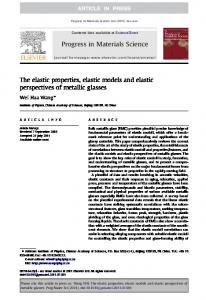
Figure 1. Low-rank force space. Non-rigid shape can be represented by means of the object elastic model and the force field acting on it. In turn, the full force field can be approximated by a low-rank basis. In this work, we simultaneously learn the elastic model (compliance matrix) and estimate the low-rank force space, while recovering shape and camera motion. In the figure we represent the full force-space and its corresponding shapes in red. The low-rank forces and shapes are shown in blue.

and the underlying forces that deform it. Interestingly, we also show its connection with the aforementioned shape and trajectory models, turning these, into physical priors too. The essence of our approach is described in Fig. 1. Let us consider N points on the object, which is deformed under the action of external forces. Following continuum mechanics, the relation between the acting forces and the deformation field can be characterized by an elastic model. Regarding the force space, we can fully define it by 3N independent forces, whose combination allows mapping the shape from a rest configuration to a wide variety of arbitrary arrangements. Yet, to represent realistic deformations, only a few of these forces, conforming a low-rank force space, are necessary. Based on this idea, we propose a new formulation of the NRSfM problem in which, given 2D point tracks, we estimate camera trajectory and force parameters (and consequently shape). Even though reasoning on the force space introduces the compliance matrix as new unknown, we are able to simultaneously solve for all parameters using Expectation Maximization (EM), with partial M steps. By thorough testing on mocap and real sequences we

1. Introduction The goal of the Non-Rigid Structure from motion (NRSfM) is to simultaneously recover the camera motion and 3D shape of a deformable object from monocular images. It is known to be a severely under-constrained problem, typically solved by introducing prior information through shape deformation models or camera trajectory constraints. Along these lines, early approaches extended the rigid factorization algorithm [37] to the non-rigid domain [7, 12, 39], and approximated the shape by a linear combination of basis estimated on-the-fly. Alternatively, other approaches have represented the evolution over time of each point on the object through a set of pre-defined trajectory basis [6, 29, 41]. Both these constraints are commonly referred to as statistical priors, as they do not have a direct physical interpretation. In this paper, we introduce a new constraint based on a low-rank force prior. This prior has a direct physical interpretation, as it models the interaction between the object 1

show that our formulation yields more accurate reconstructions than state-of-the-art shape and trajectory based methods, while providing more physical insights in terms of the elastic model of the object.

2. Related Work The inherent ambiguity of the NRSfM problem is commonly tackled by constraining the shape to lie on a low-rank space spanned by a set of deformation modes [7, 16, 17, 39]. This is further constrained by enforcing spatial [39] or temporal [7, 17] shape smoothness, or by imposing the 3D shapes to be closely aligned [22]. A number of approaches, instead constraining the shape, introduce restrictions on the trajectory of every object point using predefined bases [6, 29, 41]. There have also been recent attempts to combine low-rank shape and trajectory spaces [19, 20, 35]. All these techniques are referred to as statistically-based methods, since the low-rank representations used to condition the problem are not physically grounded. Despite their popularity, one inherent limitation of these methods is that they are very sensitive to the number of shape or trajectory modes, which needs to be carefully chosen to correctly model the deformation. A better representation of the underlying dynamics involved in non-rigid deformations can be obtained through physically-grounded models [26, 34]. Force-based kinematics [4, 13, 33], linear elastic models [24], and numerical techniques based on Finite Element Methods (FEM) for tracking [43] or 3D reconstruction [2], are just a few examples of the renewed interest in physical models. Additionally, there exist approaches in which the parameters ruling these models are learned from input data. For instance, displacement and force measurements allow recovering the Young’s modulus [44] together with the Poisson’s ratio [9]. More recently, material properties of fabrics moving under wind forces [11] or under small motions [15] are estimated from only video sequences. And vice-versa, applied forces can be recovered from 2D displacements and an estimate, up to scale, of the elastic parameters [2]. However, in all these approaches only small pieces of the full physical model (i.e., the complete stiffness matrix) are recovered. Contribution: In this paper we propose a new low-rank force model which we use to simultaneously recover camera motion, 3D shape and the full elastic model of the object. Note that the latter is specially challenging, as it involves estimating a large number of parameters, and not just the material properties such as the Young’s modulus or Poisson’s ratio. We do all this from the sole input of 2D input tracks, which may even be discontinuous due to missing data. In addition, we link our physical model to previous shape and trajectory statistical approaches, giving them a physical interpretation, too.

3. Low-rank Force Model A standard approach to reduce the ambiguity of the problem involves representing the object in low dimensional spaces. Two spaces have been considered so far, the shape and the trajectory ones. Before describing the new low-rank force space we propose, we review these previous formulations. NRS f M

3.1. Low-rank Shape and Trajectory Space The most natural way to represent time-varying shapes is by means of a low-rank shape basis. These priors are computed using either Principal Component Analysis (PCA) over training data [10, 27], applying modal analysis over a rest configuration [1, 30], or are estimated on-thefly [12, 17, 28, 39]. In particular, let us consider N 3D points on an object, being observed along T frames. If we denote by xti = [xti , yit , zit ]> the 3D coordinates of the i-th point at time t, and by st = [(xt1 )> , . . . , (xtN )> ]> the 3N dimensional representation of the shape at time t, we can compactly write the time-varying shape as a 3N×T matrix S = [s1 , . . . , sT ]. Every instant shape st can be approximated by a linear combination or Q basis shapes ˜sq : st =

Q X

˜ t ψqt ˜sq = Sψ

(1)

q=1 t > ] are the coefficients for the where ψ t = [ψ1t , . . . , ψQ ˜ = [˜s1 , . . . , ˜sQ ] is a 3N × Q matrix shape at time t, and S containing all basis shapes. By aggregating all coefficients into a Q×T matrix Ψ = [ψ 1 , . . . , ψ T ], we can finally write the factorization of the time-varying shape S as:

˜ S = SΨ.

(2)

Alternatively, we could include a shape at rest s0 in the subset of basis shapes [1, 39]. In that case, we would take ˆ = [s0 , ˜s1 , . . . , ˜sQ ], and the basis vectors ˜si , i = 1, . . . , Q S would be interpreted as 3D displacements over s0 . When representing the time-varying structure in trajectory space [6], predefined basis of a Discrete Cosine Transform (DCT) are used to span the trajectory of each object point (i.e., the rows of S). We can then factorize S as: ˜ S = ΦT,

(3)

˜ is a Q×T matrix made of Q predefined basis trawhere T jectories, and Φ is a 3N×Q matrix of trajectory coefficients.

3.2. Modeling Shapes in a Low-rank Force Space We next derive the formulation of our physics-based low-rank force model to represent the shape. We draw inspiration on the Hooke’s law, which states that the force needed to extend or compress a spring by a certain distance is proportional to that distance by a factor k, known as stiffness.

This simple model can be generalized to 3D objects with mass and volume, resulting in complex systems of partial differential equations [8] that generally do not have an analytical solution and require from numerical approximations, such as FEM. For instance, applying FEM over a shape at rest, made of N points and represented as a 3N-dimensional vector s0 , yields the following linear system: Ku = f ,

(4)

where K is the 3N×3N stiffness matrix that maps the 3N displacement vector u into a 3N -dimensional force field f . The matrix K is usually built considering a number of physical characteristics, such as material elastic properties, the type of deformation (e.g., beam bending, stress plane) and the connectivity between the nodal points, which depends on the type of element discretization (e.g., triangular, wedge, tetrahedral). Additionally, unless providing boundary conditions, K is ill-conditioned, i.e., rank(K) < 3N . Note that Eq. (4) allows computing the forces f that need to be applied onto every point of s0 to obtain a pre-defined displacement u. However, we will regard this relation in the opposite direction, that is, we seek to compute the 3D displacement when the 3D acting forces are known. In this case, we will apply the relation u = Cf , where C is a 3N × 3N compliance matrix. When boundary conditions are known this matrix is computed as C = K−1 [5, 40], and C is guaranteed to be a strictly positive-definite symmetric matrix. When boundary conditions are not available, we make use of the pseudoinverse, i.e., C = K† , but we can only assume C to be symmetric [2]. Once C is known, we can estimate a 3D displacement u for any 3D applied force vector f , and therefore a new configuration of the object shape as: s = s0 + u = s0 + Cf = C(Ks0 + f ) = C(f0 + f ), (5) where f0 = Ks0 can be interpreted as the forces applied to keep the shape at rest. We can now expand this expression to account for all T frames of a time-varying sequence: S = C[f0 + f 1 , . . . , f0 + f T ] = CF,

(6)

where F is a 3N× T matrix made of the force fields along the sequence. At this point we can introduce our low-rank force model. As it has been previously done for the shapes or point trajectories, realistic distributions of acting forces can also be approximated by a reduced number of modes. To follow the parallelism with the previous section, we consider a basis made of Q force vectors, and represent our ˜ The time-varying low-rank force field as a 3N×Q matrix F. shape can then be written as: ˜ S = CFΓ, 1

T

(7)

where Γ = [γ , . . . , γ ] is a Q×T matrix of time-varying force coefficients.

3.3. Shape-Trajectory-Force Duality A direct comparison of the low-rank shape, trajectory and force models defined in Equations (2), (3) and (7), respectively, gives the equivalence between the three representations. And most importantly, it gives a relation between two models, the shape and trajectory ones, that have thus far been considered as statistical, and our new low-rank force model, directly derived from physical relations. In particular, considering the shape-force duality, we ob˜ = CF, ˜ that is, we can write the linear subserve that S space of shapes in terms of force and elasticity parameters, and therefore, the statistical shape model does inherently encode physically-grounded properties. Similarly, we can ˜ establish a trajectory-force duality, and write that Φ = CF ˜ and T = Γ. In this case, the low-rank force model is equivalent to the trajectory coefficients, and the low-rank trajectory bases, correspond to the force coefficients. It is also worth to point that while the proposed approach has equal compaction power than shape and trajectory models, factorizing the low-rank space into a force component ˜ and a component C which encodes the elastic properties F, of the object, makes it possible to model a much wider range of object behaviors and configurations. This factorization, though, introduces an additional complexity in the learning process, as we need to discover all these terms from the sole input of 2D tracks. In the next section, we describe how we resolve this learning process, but when this is done, besides estimating shape, we could also address the inverse problem of estimating the forces necessary to obtain a specific shape configuration. This might be extremely useful in certain robotic applications dealing with the manipulation of deformable objects, or in laparoscopy surgery.

4. Learning Elastic Model, Shape and Pose In this section we describe how we introduce our lowrank force space into the formulation of the NRSfM problem, and how we then simultaneously solve for the elastic model of the object, plus the shape and camera pose.

4.1. Problem Formulation Let us consider a deformable object with N points at a time instant t, represented by a 3N vector st . Assuming an orthographic camera model, we can write the projection of the 3D points onto the image plane as a 2N vector wt : wt = Gt st + ht + nt ,

(8)

where Gt = IN ⊗ Rt has 2N × 3N size, IN is the N dimensional identity matrix, Rt are the first two rows of a full rotation matrix, and ⊗ denotes the Kronecker product. Similarly, ht = 1N ⊗ tt is a 2N vector resulting from concatenating N bidimensional translation vectors tt , and

Factor Camera Basis Coefficients Model Total number of unknowns

Full 5T 3N T 5T +3N T

Shape 5T 3N Q QT 5T + 3N Q +QT

Trajectory 5T 3N Q 5T +3N Q

Force 5T 3N Q QT 3N (3N + 1)/2 5T + 3N Q + QT +3N (3N + 1)/2

Table 1. Total number of unknowns that need to be estimated when considering the Full model, or the low-rank models in Shape, Trajectory or Force space, respectively. The results are represented in terms of the number of object points N , the number of frames T and the dimensionality Q of the low-rank space.

1N is a N -vector of ones. Finally, nt is a 2N dimensional vector of Gaussian noise. We can therefore define our problem as that of estimating, for t = 1, . . . , T , the shape st and camera pose parameters {Rt , tt }, given the observation of point tracks wt corrupted by noise nt . The total number of unobserved variables includes 3N T parameters for the shape and 5T parameters for the pose1 . Estimating all these unknowns from the only 2N T noisy observations of the point tracks is clearly an ill-posed problem. We make the problem tractable by introducing our low-rank force model and encoding the time-varying shape as: ˜ t, st = s0 + ut = s0 + CFγ

(9)

˜ are the low-rank force where C is the compliance matrix, F t vectors, and γ are the corresponding force coefficients at frame t. The projection Eq. (8) becomes: ˜ t ) + ht + nt . wt = Gt (s0 + CFγ

(10)

Note that using the low-rank force model introduces a new challenge to the problem, which is that besides having to estimate the variables involved in a standard NRSfM problem (i.e., pose, shape basis and shape coefficients, or equivalently in our framework, pose, force basis and force coefficients), we now need to learn the full elastic model C of the object. Since C remains constant along the sequence, it introduces a fixed number of unknowns independently of the number of frames T . Specifically, C is a 3N × 3N symmetric matrix, for which we only need to estimate the upper triangular part, i.e., 3N (3N + 1)/2 elements. Additionally, we still need to estimate the 5T pose parameters, 3N Q components for the low-rank force space (assuming we consider a force basis with Q components), and QT unknowns for the force coefficients. In Table 1 we summarize the total number of unknowns as a function of the parameters N (number of points), T (number of frames) and Q (dimensionality of the low-rank space) and for the full-space problem and the three low-rank versions (shape, trajectory and 1 An orthographic projection has five degrees of freedom, namely the three parameters describing the rotation matrix, plus two of the translation.

N 55 40 29 41

T 260 316 450 1,102

Q 12 11 7 10

Obs. 28,600 25,280 26,100 90,364

Full 44,200 39,500 41,400 141,056

Shape 6,400 6,376 6,009 17,760

Traj. 3,280 2,900 2,859 6,740

Force 20,095 13,636 9,837 25,386

Table 2. Total number of unknowns that need to be estimated when considering the Full model, or the low-rank models in Shape, Trajectory or Force space, respectively, for the combination of parameters N , Q and T we consider in the experimental section. The column “Obs.” refers to the number of observed variables, 2N T , corresponding to the 2D tracks of all N points along the T frames.

force). In Table 2 we give the number of unknowns for the specific combinations of N , Q and T we will use in the experimental section. Observe that for long sequences (T large), the number of unknowns of the Shape and Force subspaces become similar, while our Force-based model yields much richer information about the elastic object properties.

4.2. Probabilistic Low-Rank Force Model In order to simultaneously learn shape, pose and elastic models from 2D point tracks as described in Eq. (10), we follow a Probabilistic PCA formulation [31, 36, 38]. Broadly, this consists of two main steps. We start by writing the observations wt as a probabilistic distribution and then we estimate the parameters that maximize its likelihood using EM. We next describe the first of these steps. To estimate the distribution over the projected points wt we first assume the weight coefficients γ t to be modeled by a zero-mean Gaussian distribution γ t ∼ N (0; IQ ). These weights become latent variables that can be marginalized out and are never explicitly computed, and using Eq. (9), we can propagate their  distribution to the time-varying shapes, ˜F ˜ > C> . yielding st ∼ N s0 ; CF By also assuming the noise over the shape observations nt to follow a Gaussian distribution with variance σ 2 , i.e.,
t 2 n ∼ N 0; σ I2N , we can finally estimate that the projected points wt are also Gaussian:   ˜ t CF) ˜ > + σ 2 I2N (11) wt ∼ N Gt s0 + ht ; Gt CF(G We next explain how we perform Maximum Likelihood Estimation (MLE) on this latent variable problem using EM.

4.3. Expectation Maximization For the purpose of estimating the MLE of the distribution in Eq. (11), we use an EM algorithm in a similar way as done in [3, 38]. We denote by Θt ≡ {Rt , tt } the set of ˜ σ2 } model parameters to estimate per frame, Υ ≡ {C, F, the set of parameters to estimate along the sequence, γ t the latent variables and wt the observed data. Given the 2D trajectories of all points w = {w1 , . . . , wT }, we seek to estimate all set of parameters Θ = {Θ1 , . . . , ΘT , Υ}. The

EM algorithm iteratively estimates the maximum likelihood alternating between E-step and M -step. 4.3.1

E-Step

We initially estimate the posterior distribution over the latent variables given the current observations and model parameters. Assuming iid samples and applying the Bayes’ rule and the Woodbury’s matrix identity, it can be shown this distribution to be: p(γ t |wt , Θt , Υ) ∼ N (µtγ ; Σtγ ),

˜ µtγ =Λ(wt − Gt s0 − ht ) ; Σtγ = IQ − ΛGt CF
˜ > C Gt > (σ 2 I2N + Gt CF(G ˜ t CF) ˜ > )−1 . Λ =F M-Step

We then replace the latent variables by their expected values and update the model parameters by optimizing the negative log-likelihood function A(Θ, w) with respect to the parameters Θt , for t = 1, . . . , T , and Υ where: " T # X t t A(Θ, w) = E − log p(w |Θ , Υ) = N T log(2πσ 2 ) t=1

+

T i 1 X h t t ˜ t ) − ht k2 E kw − G (s − C Fγ 0 2 2σ 2 t=1

(13)

Note that this log-likelihood function is quadratic in all parameters we seek to estimate, and in contrast to [17, 32, 33], it does not need regularization weights. To update every parameter, we compute the corresponding partial derivative assuming the other parameters are fixed, set it to zero and solve it. The update rules we obtain are the following. Updating Elastic Model (C): To perform computations with the matrix C we need to rewrite it in vectorized form. Further, since C is symmetric, we only need to vectorize the upper triangular part of it. For this, we define the function vech(·), a generalization of the full-matrix vectorization operator vec(·). The two operators can be related by means of a so-called duplication matrix D, of size r2× r(r+1) , where 2 r is the size of the original matrix we are vectorizing [23]. For C, we have that r = 3N and we can write: vec(C) = Dvech(C) .

(14)

The inverse mapping is computed by means of the pseudoinverse, that is, vech(C) = D† vec(C). If we now set ∂A/∂vech(C) = 0, it can be shown that: vech(C) ←

T  X

 ˜ t )>⊗ (D> (Fµ ˜ t ⊗ Ir )(Gt )> Gt ) D (Fµ γ γ

t=1

×

T X t=1

γγ

t=1 T X × vec (Gt C)> (wt − Gt s0 − ht )(µtγ )>

(12)

where:

4.3.2

˜ For computing F ˜ Updating Low-Rank Force Space (F): t t t > we need to define the expectation φγγ = E[γ (γ ) ] = Σtγ + µtγ (µtγ )> . By using again the vectorized form, we can update the force space as: !−1 T X t > t > t ˜ ← (φ ) ⊗ (G C) G C vec(F)

˜ t ⊗ Ir )(Gt )> (wt − Gt s0 − ht ). D> (Fµ γ

!−1

!

t=1

Updating the Camera Pose (Rt , tt ): The camera rotation Rt needs to be updated enforcing orthonormality constraints. In order to do so we follow the iterative strategy proposed in [3], where ∂A(Rt )/∂Rt = 0 is optimized enforcing Rt to lie on the smooth manifold defined by the orthogonal group SO(3). Regarding the translation vector tt it is easy to show that it can be updated as: tt ←

N 1 X t ˜ t )i )), (w − Rt (s0,i + (CFµ γ N i=1 i

(15)

t > > ) ] , wi are 2D coordiwhere wt = [(w1t )> , . . . , (wN > > > nates, s0 = [s0,1 , . . . , s0,N ] , s0,i are 3D coordinates, and ˜ t )i is the i-th 3D point of the 3N vector CFµ ˜ t. (CFµ γ γ

Updating Noise Variance (σ 2 ): Setting ∂A(σ 2 )/∂σ 2 = 0 we can finally update the noise variance as: σ2 ←

T    1 X ˜ > Gt CFφ ˜ t tr (Gt CF) γγ 2N T t=1

+kwt−Gt s0−ht k2−2 wt−Gt s0−ht

(16)


> t ˜ t . G CFµ γ

4.4. A Comment on Scale Factor ˜ we have only constrained C When solving for C and F to be symmetric. Therefore, we could consider any sym˜ = CAA−1 F. ˜ metric and invertible matrix A such that CF A new compliance matrix CA would still be symmetric and would yield the same solution for the shape reconstruction in Eq. (9) and reprojection in Eq. (10). That is, the values of ˜ are retrieved up to a scale factor matrix. A similar C and F ˜ and γ t . ambiguity is produced between F Nevertheless, the up to scale compliance matrix C, besides yielding a correct solution to the NRSfM problem, it is also sufficient to model the full physical space. We can therefore use C to generate, up to scale, any deformation u applying a given force vector f . And vice-versa, we can obtain an scaled force field to produce a specific displacement. This kind of physical relations, are of course, not possible with previous low-rank shape and trajectory approaches. What is not possible with the compliance matrix we retrieve, though, is to directly estimate the ground truth

.

Space: PP PP Met. EM-PPCA [39] PP Seq. P P Jacky [39] 1.80(5) Face [28] 7.30(9) Flag 4.22(12) Walking [39] 11.11(10) Average error: 6.11

Shape

Trajectory

Shape-Trajectory

Force

EM-LDS [39]

MP [28]

SPM [14]

EM-PND [22]

PTA [6]

CSF2 [20]

KSTA [19]

EM-PFS

2.79(2) 6.67(2) 6.34(3) 27.29(2) 10.77

2.74(5) 3.77(7) 10.72(3) 17.51(3) 8.69

1.82(7) 2.67(9) 7.84(5) 8.02(6) 5.09

1.41 25.79 4.11 3.90 8.80

2.69(3) 5.79(2) 8.12(6) 23.60(2) 10.05

1.93(5) 6.34(5) 7.96(2) 6.39(5) 5.66

2.12(4) 6.14(8) 7.74(2) 6.36(5) 5.59

1.80(7) 2.85(5) 5.29(12) 8.54(11) 4.62

Table 3. Quantitative comparison on Mocap videos. We report e3D [%] for shape basis methods EM-PPCA [39], EM-LDS [39], MP [28] and SPM [14]; for EM-PND [22]; for the trajectory basis method PTA [6]; for shape-trajectory basis methods CSF2 [20] and KSTA [19]; and for our force basis approach denoted as EM-PFS. We have chosen the basis rank (in brackets) that gave the lowest e3D error.

values of the inherent physical parameters (e.g., Poisson’s ratio or Young’s modulus) that constitute the true stiffness matrix. For this to be possible we should perform a calibration and estimate the actual scale factor matrix, in the same line as [21] did for very specific force sensors.

4.5. Dealing with Missing Data Unlike other methods [12, 14], our approach can easily incorporate an strategy to handle incomplete measurements due to occlusions or outliers. To achieve this, during the M step of EM algorithm, we just need to optimize the expected ˆ it of the missing points. log-likelihoood of the 2D location w Since we are using a global model, we can infer their value, despite not being available. In particular we set them to: ˜ t )i ) + tt . ˆ it ← Rt (s0,i + (CFµ w γ

(17)

4.6. Initialization The optimization of Eq. (13) is a highly non-linear problem involving a large number of parameters. For this, it is important not to initialize them completely at random. In particular, we initialize the rigid motion parameters {Rt , tt } and s0 considering the scene does not deform, and we apply rigid factorization [25] as standard practice in NRSfM techniques. Regarding the compliance matrix C, we do not use any physical prior, and initially set it to the ˜ is initialized through a identity matrix. The force basis F coarse-to-fine approach, in which a noise-free version of ˜ are given, is first Eq. (10), where all parameters except F solved for one force-mode, then for two modes, and so on until estimating the Q initial modes. Once all these parameters are set, the starting value of σ 2 is directly computed from Eq. (16). Finally, when dealing with missing data we assume that both the camera motion and 3D shape deformation are smooth over time, and obtain an initial estimation ˆ it by imposing smooth trajectories, of the missing tracks w as done in [20].

5. Experimental Evaluation We now present our experimental results for different types of sequences including articulated and non-rigid motion (see videos in the supplemental material). We provide

both qualitative and quantitative results, where we compare our approach against state-of-the-art methods, using several mocap datasets with 3D ground truth. For these datasets we report the standard 3D reconstruction error, computed PT kst −st kF , where k · kF denotes the as e3D = T1 t=1 kst GT GT kF Frobenius norm, st is the estimated 3D reconstruction and stGT is the corresponding 3D ground truth. e3D is computed after aligning the estimated 3D shape with the 3D ground truth using Procrustes analysis over all T frames.

5.1. Motion Capture Data The standard way to compare NRSfM approaches is through a number of datasets with ground truth, acquired using mocap systems. We consider the following ones: the face deformation sequences Jacky and Face, from [39] and [28], respectively; Walking for articulated motion from [39], and a sparse version of Flag waving in the wind [42]. We compare our approach, denoted EM-PFS (for Expectation-Maximization on Probabilistic Force Space) against eight other methods, which use low-rank models on both shape and trajectory spaces. Among the shape space methods we consider: EM-PPCA [39], EM-LDS [39], the Metric Projections (MP) [28], the block matrix approach for SPM [14] and EM-PND [22]. Regarding the trajectorybased ones, we evaluate the DCT-based 3D point trajectory (PTA) [6]. As shape-trajectory methods we consider Column Space Fitting (CSF2) [20] and the Kernel Shape Trajectory Approach (KSTA) [19]. The parameters of these methods were set in accordance with their original papers. In our approach, the only parameter that needs to be manually set is the number Q of modes of the low-rank force space. There is no other parameter nor regularization weight that needs to be tuned. The mean 3D reconstruction errors are summarized in Table 3. Observe that our approach consistently performs either the best or among the best in all sequences, and in average is the one with smaller error. In particular note that we slightly outperform SPM [14] and KSTA [19], which are acknowledged to be at the top of the state-of-the-art in lowrank based models. And most importantly, we do not only solve for the NRSfM problem, but we additionally provide an estimation of the full elastic model of the object.

Figure 2. Actress sequence. Top: 2D tracking data (green circles) and reprojection (red dots) of the reconstructed 3D shape. Middle: Camera and side-views of the reconstructed shapes. Bottom: Same views using EM-PND [22].

Figure 4. Back sequence. Top: See caption of Fig. 2. Bottom: Side view of the reconstructed shape.

Figure 5. ASL sequence. Top: See caption of Fig. 2. Bottom: Camera frame and side-views of the reconstructed 3D shape. Blue circles correspond to missing points. Best viewed in color. Figure 3. Beating heart sequence. Top: See caption of Fig. 2. Middle: Reconstructed 3D shape, color code such that reddish areas indicate larger displacements. Bottom: Reconstructed 3D shape, using the original texture. Best viewed in color.

5.2. Real Videos We have also evaluated our approach on several real sequences, which despite not having ground truth, allow a qualitative evaluation in different real-world scenarios and under the presence of structured occlusions, where other approaches are prone to fail [14]. First, we process the actress sequence, with 102 frames showing a woman talking and moving her head. The point tracks were provided by [7]. Figure 2 shows the 3D reconstruction, appropriately rotated according to the estimated pose. We also show the results of the EM-PND [22], known to be very accurate except for situations like this sequence, in which the camera rotation is small. For the beating heart sequence, of 79 frames and acquired during bypass surgery2 , we use the outlier-free point tracks of [18], computed using optical flow. Figure 3 shows the 3D reconstruction we obtain, where one of the main challenges is that the movement of the camera is very small. This especially penalizes trajectory-based methods. The color-coded reconstructions, representing the amount of deformation, show that we can recover the rhythmic deformations of the heart, while learning its elastic model. 2 Sequence

available from: http://hamlyn.doc.ic.ac.uk/vision

Figure 4 shows the reconstruction of the back of a person. Point tracks are obtained from [32]. Again, one of the difficulties of this sequence is to deal with small camera motions, which our approach handles without much difficulty. Finally, we have also processed an ASL sequence of an American Sign Language (ASL), consisting of a person moving the head while talking and hand gesturing. The goal is to reconstruct the face which, in some frames is partially occluded by the hand or by the own face rotation. The sequence, from [20], has 114 frames and 11.5% of missing data. Fig. 5 shows two views per frame of the estimated 3D shape. Note that even when occlusions appear, our model provides a correct estimation for the occluded shape. While this reconstruction is very similar to that obtained by [20], SPM [14], our closer competitor in the mocap data experiments of Table 3, is not able to handle missing data.

5.3. Elastic Model Estimation The distinguishing contribution of our approach is that besides estimating the shape and camera trajectory, we provide an estimation of the elastic model of the object C, and ˜ (with the corresponding force coa low-rank force space F efficients Γ). Additionally, as discussed in Sect. 3.3, once we have estimated these parameters, we can directly compute the equivalence between the force, shape and trajectory spaces. Concretely, the low-rank shape space has been ˜ = CF, ˜ and the low-rank trajectory space shown to be S ˜ = Γ. In Fig. 6 we plot these equivalences for the exT ample of the actress sequence introduced previously. On

f1 f2 f3 f4

Full Physical Space (C)

fr1 fr2 fr3 fr4

Force

0 20

Shape

Degrees of freedom

40 60 80 100 120 140 160 180

Trajectory

200 0 5

5

5

5

5

0

0

0

0

0

−5 0

20

40

60

80

100

−5 0

20

40

60

80

−5 100 0

20

40

60

80

−5 100 0

20

40

60

80

−5 100 0

50

100

150

200

Degrees of freedom

20

40

60

80

100

Number of frame t Number of frame t Number of frame t Number of frame t Number of frame t

Figure 6. Spaces comparison. Equivalence between the force, shape and trajectory spaces using the actress sequence, with rank Q = 5. Top: Modes in the force space. Middle: Modes in the shape space. Bottom: Modes in the trajectory space.

top we plot the first five force modes, as vectors overlaying the shape at rest. Observe that the larger magnitudes of the modes concentrate around the mouth, which is the part of the face undergoing larger deformations. On the center, we plot the equivalent shape basis we retrieve. Again, although it is difficult to appreciate from non-overlapping images, note the subtle differences between the configuration of each mode, and again, particularly around the area of the mouth. The bottom-most plot, depicts the first five trajectory modes, with size equal to the sequence length. The theoretical modes used in the trajectory-based methods correspond to the sinusoidal functions of a DCT. Note that the first mode we estimate from our force-space, quite resembles such a function. In Fig. 7 we demonstrate that the compliance matrix we estimate allows recovering the full physical space. For instance the four face configurations we plot on the left are produced by applying specific forces f and computing the resulting deformations u via the relation u = Cf . Each face corresponds to the product of the compliance matrix, shown in the center of the figure, by one of the force vectors f1 , f2 , f3 , f4 depicted on the right, plus the shape at rest. Observe that with this force model we can generate shape configurations (e.g., winking one or two eyes, mouth wide open) that would be hard or impossible to obtain using lowrank shape and trajectory spaces unless similar shapes are explicitly observed (in shape-based methods) or they use a very large number of modes (in trajectory-based methods). In contrast, using the physical space we propose, we can produce these shapes even when they have not been observed and directly from the elastic model we have learned. Additionally, note how the forces f1 , f2 , f3 , f4 necessary to produce these shape configurations are smooth (their color coded components do not abruptly change). This would not happen if we had used a random symmetric compli-

Figure 7. Full physical space estimation for the actress sequence. Once the compliance matrix is learned, we can define any shape in the full physical space. Left: Four shapes obtained from the estimated C. Center: Recovered C. Right: f1 , f2 , f3 , f4 , are the forces necessary to obtain the shape configurations on the left from C, the estimated compliance matrix. f1r , f2r , f3r , f4r , are the forces necessary to obtain the same shape configurations, but from a random symmetric compliance matrix. Best viewed in color.

ance matrix. This matrix would also solve allow minimizing Eq. (13), but the resulting forces f1r , f2r , f3r , f4r would not be quite realistic. We plot these forces, on the rightmost of Fig. 7. Note how their values evidence sharp changes, indicating that a random compliance matrix would not appropriately model the underlying physics of the object.

6. Conclusions In this paper we have formulated the NRSfM problem using a new low-rank force model. From only 2D point tracks, besides recovering shape and camera motion, this approach also provides an estimation of an elastic model of the object, allowing for rich physical interpretations of the dynamics in terms of force and displacement. Additionally, we have shown the connections of our force-model to the shape and trajectory-based spaces used so far. The results demonstrate that the proposed technique is applicable to a wide variety of real-world deformations and materials, without requiring any prior knowledge about the physical or geometric object properties. We obtain state-of-the-art performance in reconstruction accuracy, while also providing an estimation of the object elastic model. Yet, this model is recovered up to scale. In the future, we plan to retrieve the true elastic model by including certain constraints into our optimization. By doing this from just a monocular video would be a major step in engineering mechanics, which usually rely on complex laboratory procedures for obtaining such models.

Acknowledgments This work was partly funded by the MINECO projects DIP2012-32168 and TIN2014-58178-R; by the ERA-net CHISTERA project VISEN PCIN-2013-047; and by a scholarship FPU12/04886 of the Spanish MECD. We also thank Paulo Gotardo for making their data available.

References [1] A. Agudo, L. Agapito, B. Calvo, and J. M. M. Montiel. Good vibrations: A modal analysis approach for sequential nonrigid structure from motion. In CVPR, 2014. [2] A. Agudo, B. Calvo, and J. M. M. Montiel. Finite element based sequential bayesian non-rigid structure from motion. In CVPR, 2012. [3] A. Agudo, J. M. M. Montiel, L. Agapito, and B. Calvo. Online dense non-rigid 3D shape and camera motion recovery. In BMVC, 2014. [4] A. Agudo and F. Moreno-Noguer. Simultaneous pose and non-rigid shape with particle dynamics. In CVPR, 2015. [5] A. Agudo, F. Moreno-Noguer, B. Calvo, and J. M. M. Montiel. Sequential non-rigid structure from motion using physical priors. TPAMI, to appear, 2015. [6] I. Akhter, Y. Sheikh, S. Khan, and T. Kanade. Non-rigid structure from motion in trajectory space. In NIPS, 2008. [7] A. Bartoli, V. Gay-Bellile, U. Castellani, J. Peyras, S. Olsen, and P. Sayd. Coarse-to-fine low-rank structure-from-motion. In CVPR, 2008. [8] K. J. Bathe. Finite element procedures in Engineering Analysis. Prentice-Hall, 1982. [9] M. Becker and M. Teschner. Robust and efficient estimation of elasticity parameters using the linear finite element method. In SIMVIS, 2007. [10] V. Blanz and T. Vetter. A morphable model for the synthesis of 3D faces. In SIGGRAPH, 1999. [11] K. L. Bouman, B. Xiao, P. Battaglia, and W. T. Freeman. Estimating the material properties of fabric from video. In ICCV, 2013. [12] C. Bregler, A. Hertzmann, and H. Biermann. Recovering non-rigid 3D shape from image streams. In CVPR, 2000. [13] M. Brubaker, L. Sigal, and D. Fleet. Estimating contact dynamics. In ICCV, 2009. [14] Y. Dai, H. Li, and M. He. A simple prior-free method for non-rigid structure from motion factorization. In CVPR, 2012. [15] A. Davis, K. Bouman, J. Chen, M. Rubinstein, F. Durand, and W. Freeman. Visual vibrometry: Estimating material properties from small motions in video. In CVPR, 2015. [16] K. Fragkiadaki, M. Salas, P. Arbel´aez, and J. Malik. Grouping-based low-rank trajectory completion and 3D reconstruction. In NIPS, 2014. [17] R. Garg, A. Roussos, and L. Agapito. Dense variational reconstruction of non-rigid surfaces from monocular video. In CVPR, 2013. [18] R. Garg, A. Roussos, and L. Agapito. A variational approach to video registration with subspace constraints. IJCV, 104(3):286–314, 2013. [19] P. F. U. Gotardo and A. M. Martinez. Kernel non-rigid structure from motion. In ICCV, 2011. [20] P. F. U. Gotardo and A. M. Martinez. Non-rigid structure from motion with complementary rank-3 spaces. In CVPR, 2011. [21] M. Hwangbo and T. Kanade. Factorization-based calibration method for MEMS inertial measurement unit. In ICRA, 2008.

[22] M. Lee, J. Cho, C. H. Choi, and S. Oh. Procrustean normal distribution for non-rigid structure from motion. In CVPR, 2013. [23] J. R. Magnus and H. Neudecker. Matrix Differential Calculus with Applications in Statistics and Econometrics. John Wiley and Sons: Chichester/New York, 1988. [24] A. Malti, R. Hartley, A. Bartoli, and J. H. Kim. Monocular template-based 3D reconstruction of extensible surfaces with local linear elasticity. In CVPR, 2013. [25] M. Marques and J. Costeira. Optimal shape from estimation with missing and degenerate data. In WMVC, 2008. [26] D. Metaxas and D. Terzopoulos. Shape and nonrigid motion estimation through physics-based synthesis. TPAMI, 15(6):580–591, 1993. [27] F. Moreno-Noguer and J. M. Porta. Probabilistic simultaneous pose and non-rigid shape recovery. In CVPR, 2011. [28] M. Paladini, A. Del Bue, M. Stosic, M. Dodig, J. Xavier, and L. Agapito. Factorization for non-rigid and articulated structure using metric projections. In CVPR, 2009. [29] H. S. Park, T. Shiratori, I. Matthews, and Y. Sheikh. 3D reconstruction of a moving point from a series of 2D projections. In ECCV, 2010. [30] A. Pentland and B. Horowitz. Recovery of nonrigid motion and structure. TPAMI, 13(7):730–742, 1991. [31] S. Roweis. EM algorithms for PCA and SPCA. In NIPS, 1998. [32] C. Russell, J. Fayad, and L. Agapito. Energy based multiple model fitting for non-rigid structure from motion. In CVPR, 2011. [33] M. Salzmann and R. Urtasun. Physically-based motion models for 3D tracking: A convex formulation. In ICCV, 2011. [34] S. Sclaroff and A. Pentland. Physically-based combinations of views: Representing rigid and nonrigid motion. In MNRAO, 1994. [35] T. Simon, J. Valmadre, I. Matthews, and Y. Sheikh. Separable spatiotemporal priors for convex reconstruction of timevarying 3D point clouds. In ECCV, 2014. [36] M. E. Tipping and C. M. Bishop. Mixtures of probabilistic principal component analysers. NC, 11(2):443–482, 1999. [37] C. Tomasi and T. Kanade. Shape and motion from image streams under orthography: A factorization approach. IJCV, 9(2):137–154, 1992. [38] L. Torresani, A. Hertzmann, and C. Bregler. Learning nonrigid 3D shape from 2D motion. In NIPS, 2004. [39] L. Torresani, A. Hertzmann, and C. Bregler. Nonrigid structure-from-motion: estimating shape and motion with hierarchical priors. TPAMI, 30(5):878–892, 2008. [40] L. V. Tsap, D. B. Goldof, and S. Sarkar. Nonrigid motion analysis based on dynamic refinement of finite element models. TPAMI, 22(5):526–543, 2000. [41] J. Valmadre and S. Lucey. General trajectory prior for nonrigid reconstruction. In CVPR, 2012. [42] R. White, K. Crane, and D. Forsyth. Capturing and animating occluded cloth. In SIGGRAPH, 2007. [43] S. Wuhrer, J. Lang, and C. Shu. Tracking complete deformable objects with finite elements. In 3DIMPVT, 2012. [44] Y. Zhu, T. J. Hall, and J. Jiang. A finite-element approach for young modulus reconstruction. TMI, 22(7):890–901, 2003.