Learning Shape Segmentation Using Constrained Spectral Clustering ...

Learning Shape Segmentation Using Constrained Spectral Clustering and Probabilistic Label Transfer Avinash Sharma, Etienne von Lavante, and Radu Horaud INRIA Grenoble Rhˆone-Alpes, Montbonnot Saint-Martin, France

Abstract. We propose a spectral learning approach to shape segmentation. The method is composed of a constrained spectral clustering algorithm that is used to supervise the segmentation of a shape from a training data set, followed by a probabilistic label transfer algorithm that is used to match two shapes and to transfer cluster labels from a training-shape to a test-shape. The novelty resides both in the use of the Laplacian embedding to propagate must-link and cannotlink constraints, and in the segmentation algorithm which is based on a learn, align, transfer, and classify paradigm. We compare the results obtained with our method with other constrained spectral clustering methods and we assess its performance based on ground-truth data.

1 Introduction In this paper we address the problem of segmenting shapes into their constituting parts with emphasis onto complex 3D articulated shapes. These shapes are difficult to describe in terms of their parts, e.g., body parts of humans, because there is a large variability within the same class of perceptually similar shapes. The reasons for this are numerous: changes in pose due to large kinematic motions, local deformations, topological changes, etc. Without loss of generality we will represent 3D shapes with meshes which can be viewed as both 2D discrete Riemannian manifolds and graphs. Therefore, shape segmentation can be cast into the problem of graph partitioning for which spectral clustering (SC) algorithms [1] provide tractable solutions. Nevertheless, unsupervised spectral clustering algorithms will not always yield satisfactory shape segmentation results for the following reasons: Distances between vertices are only locally Euclidean (manifold structure), the graph has bounded connectivity (sparseness), and the number of edges meeting at each vertex is almost the same through the graph (regular connectivity). Manifoldness will exclude methods that need a fully-connected affinity matrix. While sparseness makes shape-graphs good candidates for Laplacian embedding [2,3], the usual spectral clustering assumptions do not hold in the case of regular connectivity. First, the Laplacian matrix of a shape-graph cannot be viewed as a slightly perturbed version of the ideal case1 , namely a number of strongly connected components that are only weakly interconnected [1]. Second, there is no eigengap and hence there is no simple way to determine the number of clusters. Third, the eigenvectors associated with the smallest non-null eigenvalues cannot be viewed as relaxed indicator vectors [1]. 1

In the ideal case the between-cluster similarity cost is exactly 0.

K. Daniilidis, P. Maragos, N. Paragios (Eds.): ECCV 2010, Part V, LNCS 6315, pp. 743–756, 2010. c Springer-Verlag Berlin Heidelberg 2010

744

A. Sharma, E. von Lavante, and R. Horaud

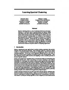
Fig. 1. First stage: Constrained spectral clustering (CSC) which takes as input a mesh (or more generally a graph) together with a sparse set of must-link (dashed lines) and cannot-link (full lines) constraints (a). These constraints are propagated using the commute-time distance (b). Spectral clustering is applied to a modified graph Laplacian (c). Second stage: Probabilistic label transfer (PLT). Shape segmentation is performed via vertex-to-vertex matching (d) and label transfer (e).

In this paper we propose a learning approach to shape segmentation via a two-stage method, e.g., fig. 1. First we introduce a new constrained spectral clustering (CSC) algorithm which takes as input a shape-graph Gtr from a training set. Gtr contains unlabeled vertices as well as must-link and cannot-link constraints between pairs of vertices, fig. 1-(a). These constraints are propagated, using the unnormalized Laplacian embedding and the commute-time distance (CTD), such that edge-weights corresponding to within-cluster connectivities are strengthened while those corresponding to betweencluster connectivities are weakened, fig. 1-(b). This modified embedding yields improved shape segmentation results than the initial one, e.g., fig. 1-(c), because it better fits into the theoretical requirements of spectral clustering [1]. Second, we consider shape alignment based on vertex-to-vertex graph matching as a way to probabilistically transfer labels from a training-set of segmented shapes to a test-set of unsegmented ones. We consider a shape-graph Gtest from a test set. The segmentation of Gtest is carried out via a new probabilistic label transfer (PLT) method that computes a point-to-point mapping between the embedding of Gtr and Gtest , e.g., fig. 1-(d). This completely unsupervised matching is based on [4,5] and allows to transfer labels from a segmented shape to an unsegmented one. Consequently, the vertices of Gtest can be classified using the segmentation trained with Gtr , fig. 1-(e). While the spectral graph matching is appealing [6], it adds an extra difficulty because of the ambiguity in the definition of spectral embeddings up to switching between eigenvectors corresponding to eigenvalues with multiplicity and changes in their sign [4,7]. This is particularly critical in the presence of symmetric shapes [8]. Unsupervised segmentation of articulated shapes is a well investigated problem and one can find a quantitative comparison of recent non-spectral methods in [9]. However, the spectral methods are natural choice for pose-invariant segmentation as they exploit the inherent manifold structure of the mesh representation to embed the shape in an isometric space. For the reasons already mentioned in the introduction, the results of simple spectral clustering (SC) are unsatisfactory ([1] for both a tutorial and

Learning Shape Segmentation Using Constrained Spectral Clustering

745

comprehensive study). Therefore, more recent methods, such as those by Reuter [10] and Zhang [11], also take the topological features of a shape in its embedded space into account and can achieve this way impressive segmentation results. However, these methods do not provide intuitive means to include constraints in a semi-supervised framework. Regarding semi-supervised spectral methods, we distinguish between semi-supervised and constrained spectral clustering methods: With semi-supervised spectral methods we consider algorithms which attempt to find good partitions of the data given partial labels. In [12] labeled data information is propagated to nearby unlabeled data using a probabilistic label diffusion process, which needs an extra time parameter that must be specified in advance [13,14,7]. In [15] the labeled data are used to learn a classifier that is then used to sort the unlabeled data. These methods work reasonably well if there are sufficient labeled data or if the data can be naturally split into clusters. Furthermore, these methods were only applied to synthetic “toy” data and their extension to graphs that represent shapes may not be straightforward. Constrained clustering methods use prior information under the form of pairwise must-link and cannot-link constraints, and were first introduced in conjunction with constrained K-means [16]. Subsequently, a number of solutions were proposed that consist in learning a distance metric that takes into account the pairwise relationships; This generally leads to convex optimization [17,18]. Since K-means is a ubiquitous post-processing step with almost any SC technique, it is tempting to replace it with constrained K-means. However, this does not take full advantage of the graph structure of the data where edges naturally encode pairwise relationships. Recently, metric learning has been extended to constrained spectral clustering leading to quadratic programming [19]. The semi-supervised kernel K-means method [20] incorporates constraints by adding reward and penalty terms to the cost function to be minimized. Another way to incorporate constraints into spectral methods is to modify the affinity matrix of a graph using a simple rule: Edges between must-link vertex-pairs are set to 1 and edges between cannot-link pairs are set to 0 [21]. Despite its simplicity, this method is not easily extendible to our case due to graph sparsity: one has to add new edges (with value 1) and to remove some other edges. This will modify the graph’s topology and hence it will be difficult to use the segmentation learned on one shape in order to segment another shape. All methods described above need a large number of constraints to work well, which is a major drawback, as it is desirable to work with a small set of sparse constraints. We note that the issue of constraint propagation is not well studied: The transitivity property of the must-link relationship has already been explored [22] but this cannot be used with the cannot-link relationship which is not transitive. 1.1 Paper Contributions This paper has two contributions: A new constrained spectral clustering method that uses the unnormalized Laplacian embedding to propagate pairwise constraints and a modified Laplacian embedding to cluster the data, and a new shape segmentation method based on spectral graph matching and on a novel probabilistic label-transfer process.

746


We exploit the properties of the unnormalized graph Laplacian [3,1] which embeds the graph into an isometric space armed with a metric, namely the Euclidean commutetime distance (CTD) [23,14]. Unlike the diffusion maps that are parameterized by a discrete time parameter, which acts as a scale, [13], the CTD reflects the connectivity of two graph vertices: All possible paths of all lengths. We build on the idea of modifying the weighted adjacency matrix of a graph using instance level constraints on vertex-pairs [21]. We provide an explicit constraint propagation method that uses the Euclidean CTD to densify must-link and cannot-link relationships within small volumes lying between constrained data pairs. We show that the modified weighted adjacency matrix thus obtained can be used to construct a modified Laplacian. The latter respects the topology of the initial graph but with a distinct geometric structure that have the presence of dense graph lumps, which is a direct consequence of the constraint propagation process: This makes it particularly well suited for clustering. We introduce a shape segmentation method based on a learn, align, transfer, and classify paradigm. This introduces an important innovation, namely that one can perform the training on one data-set and then classify a completely different data-set on the premise that the two sets are approximately isomorphic. Our probabilistic label transfer algorithm is robust to topological noise as we consider dense soft correspondences between two shapes. We compare our CSC algorithm with several other methods recently proposed in the literature, and we evaluate it against ground-truth segmentations of both simulated and real shapes. We note that the existing CSC methods have not been applied to articulated shapes which are rather complex discrete Riemannian manifolds. Real shapes gathered with scanners and cameras are very challenging dataset. As already mentioned, these manifold data are very difficult to cluster due to the regularity of the associated graph.

2 Laplacian Embeddings and Their Properties We consider an undirected weighted graph G = {V, E, A} where V(G) = {v1 , . . . , vn } is the vertex set, E(G) = {eij } is the edge set, and the entries of the weighted adjacency matrix A are: aii = 0, aij > 0 whenever two vertices are adjacent, i.e., vi ∼ vj , and aij = 0 otherwise. In the case of 2D manifolds, a vertex vi corresponds to a 3D point v i . Let 0 < amin ≤ aij ≤ amax ≤ 1. Since our graphs correspond to a uniform surface discretization, it is realistic to assume that the weights vary within a small interval [amin , amax ]. Without loss of generality we consider Gaussian weights i.e. aij = exp(−d2ij /σ 2 ). We briefly recall the following definitions: the degree matrix D = Diag [di . . . dn ], the n-dimensional degree vector d = (d1 . . . dn ) , with di = i∼j aij . The following Laplacian matrices are used in spectral clustering [1]: The unnormalized Laplacian L = D − A, the normalized Laplacian LN = D−1/2 LD−1/2 , and the random-walk Laplacian LR = D−1 L. Both L and LN are symmetric semi-positive definite, hence their eigenvalues are non-negative and their eigenvectors form an orthonormal vector basis of Rn . From the similarity LR = D−1/2 LN D1/2 one can easily characterize the eigenspace of the random-walk graph Laplacian. It has been recently shown that both L and LR are well suited for spectral clustering [1]. In this section we describe some


747

interesting properties of the unnormalized Laplacian which justify its use for both the tasks of clustering and of matching. The L-embedding. Let Lu = λu, denote Λ = Diag [λ2 . . . λp+1 ], and let U = [u2 . . . up+1 ] be the n × p matrix formed with the p smallest non-null eigenvectors of L, hence U U = Ip . We have as well λ1 = 0 and u1 = 1 (a vector with all entries equal to 1). The columns of U form an orthonormal basis that span an embedded space Rp ⊂ Rn perpendicular to 1. Hence, we have the following property: n

ui (vj ) = 0, ∀i, 2 ≤ i ≤ p + 1

(1)

j=1

where we introduced the notation ui (vj ) for the j-th entry of vector ui in order to emphasize that each eigenvector is an eigenfunction mapping the graph’s vertices onto real numbers. The Euclidean embedding of the graph’s nodes that we will use are the column vectors of the p × n matrix X defined by: X = Λ−1/2 U = [x1 . . . xj . . . xn ]

(2)

This is also known as the commute-time embedding [14]. From the orthonormality of the eigenvectors and from (1) we obtain: −1/2

−λi

−1/2

< ui (vj ) < λi

, ∀j, 1 ≤ j ≤ n

(3)

The L-embedding. So far we described the properties of spectral embeddings that correspond to graphs that contain only unlabeled vertices. As it will be explained in the next section, the presence of pairwise constraints could lead to a modified Laplacian embedding and in this paragraph we describe the rationale of this modified spectral representation. We suppose that pairwise constraints are provided and we consider one such vertex-pair. Two situations can occur: (i) the two vertices are adjacent or, more generally, (ii) the two vertices are connected by one or several graph paths. While the former situation leads to simply modifying the edge weights of the corresponding pairs, the latter is more problematic to implement because it involves some form of constraint propagation and it constitutes the topic of section 3. To summarize, the presence of constraints leads to modifying some of the edge weights in the graph. We denote the We also obtain a modified degree matrix D and a modified adjacency matrix with A. modified unnormalized Laplacian L: =D −A L

(4)

This leads to modified Euclidean coordinates: = [ =Λ −1/2 U j . . . x n] x1 . . . x X

(5)

The initial graph can therefore be represented with two different embeddings, the exact geometry of the embedded space depending on the edge weights. Notice, that there is a one-to-one correspondence between the columns of X and of X.

748


3 Propagating Pairwise Constraints In a constrained clustering task instance-level constraints are available. In practice, it is convenient to be able to cope with a sparse set of constraints. The counterpart is that they are not easily exploitable: propagating these constraints over a manifold (or more generally over a graph) is problematic. In this section we describe a constraint propagation method that uses the L-embedding and the associated Euclidean commutetime distance (CTD). As already mentioned, must-link and cannot-link constraints were successfully incorporated in several variant of the K-means algorithm [16,17,18]. However, these methods did not incorporate constraint propagation. Rather than modifying the K-means step of spectral clustering, we incorporate a constraint-propagation process directly into the L-embedding, thus fully exploiting the properties outlined in the previous section. Consider a subset of the set of graph vertices S = {¯ vi }, S ⊂ V from which we build two sets of constraints: A must-set M ⊂ S × S and a cannot-set C ⊂ S × S. Vertex pairs from the must-set should be assigned to the same cluster while vertex pairs from the cannot-set should be assigned to different clusters. Notice that the cardinality of these sets is independent of the final number of clusters. Also, it is necessary neither to provide must links for all the clusters, nor to provide cannot links across all cluster pairs. A straightforward strategy for enforcing these constraints consists in modifying the weights aij associated with adjacent vertex-pairs that belong either to M or to C, such that aij is replaced with a ˜ij = 1 if (¯ vi , v¯j ) ∈ M and a ˜ij = ε if (¯ vi , v¯j ) ∈ C, where ε is a small positive number. We recall that 0 < amin ≤ aij ≤ amax ≤ 1. Notice that for graphs corresponding to regular meshes, the edge-weight variability is small. Since the set S is composed of sparsely distributed vertices, the pairs (¯ vi , v¯j ) do not necessarily correspond to adjacent vertices. Hence, one has to propagate the initial must-link and cannot-link constraints to nearby vertex pairs. We propose to use the commute-time distance (CTD) already mentioned. The CTD is a well known quantity in Markov chains [24]. For undirected graphs, it corresponds to the average number of (weighted) edges that it takes, starting at vertex vi , to randomly reach vertex vj for the first time and go back. The CTD has the interesting property that it decreases as the number of paths connecting the two nodes increases and when the lengths of the paths

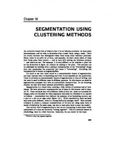
Fig. 2. Propagating constraints. (a): Constraint placement onto the initial graph, two must-links (dashed lines) and one cannot-link; (b): The L-embedding used for constraint propagation. (c): The propagated constraints are shown on the graph. (d): The new embedding obtained with the modified Laplacian L.


749

Fig. 3. The CSC algorithm applied to the the dog and to the flashkick data (Note: unlike the results in Table 1, we seek here for flashkick 14 segments). Initial graphs and manually placed constraints (a), (d); Constraint propagation (b), (e); Final clustering results (c), (f).

decrease. We prefer the CTD to the shortest-path geodesic distance in the graph because it captures the connectivity structure of a small graph volume rather than a single path between two vertices. The CTD is the integral of the diffusion distances over all times. Hence, unlike the latter, the former does not need the free parameter t to be specified [13,14,7]. Indeed, the scale parameter introduces an additional difficulty because different vertex-pairs may need to be processed at different scales. The commute-time distance [23] between two vertices is an Euclidean metric and it can be written in closed form using the L-embedding, i.e., eq. (2): d2CTD (vi , vj ) = xi − xj 2

(6)

The CTD will allow us to propagate must-link and cannot-link constraints within small graph volumes, e.g., fig. 2. We briefly describe the propagation of must-link constraints. For each pair (¯ vi , v¯j ) ∈ M with embedded coordinates xi and xj : We consider the hypersphere centered at (xi + xj )/2 with diameter given by (6) and we build a subset Xs ⊂ X that contains embedded vertices lying in this hypersphere. We build a subgraph Gs ⊂ G having as vertices the set Xs = {vi }ri=1 corresponding to Xs . Finally, we modify the ˜ij = 1. There is an equivalent procedure for the propweights aij of the edges of Gs : a agation of cannot-link constraints. In order to preserve the topology of the modified graph, in this case the weights are set to a small positive number, i.e., the modified weight of a cannot-edge is a ˜ij = ε. Hence the proposed CSC algorithm, fig. 3: Algorithm 1. Constrained Spectral Clustering (CSC) input : Unnormalized Laplacian L of a shape-graph G, a must-link set M, a cannot-link set C, the number of cluster k to construct. output : A set of binary variables Δ = {δil } assigning a cluster label l to each graph vertex vi . 1: Compute the L-embedding of the graph using the p first non-null eigenvalues and eigenvectors of L, p ≥ k. 2: Propagate the M and C constraints, modify the adjacency matrix of G and build the modified using eq. (4). Laplacian L 3: Compute the L-embedding using the k first non-null eigenvalues and eigenvectors of L. in 4: Assign a cluster label l to each graph vertex vi by applying K-means to the points X eq. (5).

750


4 Shape Segmentation via Label Transfer The CSC algorithm that we just described is applied to a shape-graph Gtr such that the latter is segmented into k clusters. Given a second shape Gtest we wish to use the segmentation result obtained with Gtr to segment Gtest . Therefore, the segmentation of Gtest can be viewed as an inference problem, where we seek a cluster label for each one of its vertices conditioned by the segmentation of Gtr . We formulate this label inference problem in a probabilistic framework and adopt a generative approach where we model the conditional probability of assigning a label to a test shape vertex. More formally, let Xtr and Xtest be the L-embeddings of the two shapes with n and m vertices respectively, i.e., eq. (2). We introduce three sets of hidden variables: S = {s1 , . . . , sm } which assign each test-shape vertex to its cluster, R = {r1 , . . . , rn } which assign each train-shape vertex to its cluster, and Z = {z1 , . . . , zm }, which assign a test-shape vertex to a train-shape vertex. Then the posterior probability ∈ Xtest can be of assigning a cluster label l ∈ {1, . . . , k} to a test-shape vertex xtest i written as: n P (rj = l|xtrj )P (zi = j|xtest (7) P (si = l|xtest i ) = i ), j=1

l|xtrj )

is the posterior probability of assigning a label l to a train-shape Here, P (rj = vertex xtrj , conditioned by the train-shape vertex. Similarly, P (zi = j|xtest i ) is the posterior probability of assigning train-shape vertex xtrj to test-shape vertex xtest and can i be termed as soft assignment. We propose to replace the posteriors P (rj = l|xtrj ) with hard assignments, namely the output of the CSC algorithm: P (rj = l|xtest j ) = δjl

(8)

The estimation of the posteriors P (zi = j|xtest i ) is an instance of graph matching in the spectral domain which is a difficult problem in its own right, especially in the presence of switches between eigenvectors and changes in their sign. The graph/shape matching task is further complicated when the two graphs are not isomorphic and when they have different numbers of vertices. We adopted the articulated shape matching method proposed in [4,5] to obtain these soft assignments. This method proceeds in two steps. The first step uses the histograms of the k first non-null eigenvectors of the normalized Laplacian matrix to find an alignment between the Euclidean embeddings of two shapes. The second step registers the

Fig. 4. Clustering obtained with CSC (a), (d); vertex-to-vertex probabilistic assignment between two shapes (b), (e); The result of segmenting the second shape based on label transfer (c), (f)


751

two embeddings using the expectation-maximization (EM) algorithm and selects the best vertex-to-vertex assignment based on the maximum a posteriori probability (MAP) of a vertex from one shape to be assigned to a vertex from the other shape. In order to fit to our methodological framework, we introduce two important modifications to the technique described in [4]: 1. We use the unnormalized Laplacian. This is justified by the properties of the Lembeddings which where described in detail in section 2. In particular, the property (3) facilitates the task of comparing the histograms of two eigenvectors. 2. We do not attempt to find the best one-to-one assignments based on the MAP criterion. Instead, we keep all the assignments and hence we rely on soft rather than hard assignments. The resulting shape matching algorithm will output the desired posterior probabilities P (zi = j|xtest i ) = pij , ∀1 ≤ i ≤ m. From (7) and (8) we obtain the following expression that probabilistically assigns a vertex of Gtest to a cluster of Gtr : γil = arg max 1≤l≤k

n

pij δjl

(9)

j=1

This corresponds to the maximum posterior probability of a test-shape vertex to be assigned to a train-shape cluster conditioned by the test-shape vertex and by the trainshape-to-test-shape soft assignments of vertices. The proposed segmentation method is summarized in algorithm 2. Fig. 4 illustrates the PLT method on two examples. Algorithm 2. Probabilistic Label Transfer (PLT) input : L-embeddings Xtr and Xtest of train and test shape-graphs Gtr and Gtest ; a set of binary variables Δ = {δjl } assigning a cluster label l to each vertex xtrj ∈ Xtr . ∈ output : A set of binary variables Γ = {γil } assigning a cluster label l to each vertex xtest i Xtest . 1: Align two L-embeddings Xtr and Xtest using the histogram alignment method [4]. to every train 2: Compute the posterior probability pij of assigning each test graph vertex xtest i graph vertex xtrj using the EM based rigid point registration method proposed in [5]. using the eq.(9). 3: Find the cluster label l for each test graph vertex xtest i

5 Experiments and Results We evaluated the performance of our approach on 3D meshes, consisting of both synthetic 2 and real articulated shapes 3 having a wide range of variability in terms of mesh topology, kinematic poses, noise and scale. Particularly, the data acquired by multicamera systems are non-uniformly sampled and there are major topological changes in 2 3

http://tosca.cs.technion.ac.il/book/resources_data.html http://people.csail.mit.edu/drdaniel/mesh_animation/index.html http://4drepository.inrialpes.fr/public/datasets http://www.ee.surrey.ac.uk/CVSSP/VisualMedia/ VisualContentProduction/Projects/SurfCap

752


between the various kinematic poses, e.g., fig. 1(c). We have generated manual segmentations of all the employed meshes as a ground truth for the quantitative evaluation of our approach. As a consequence of this, one-to-one correspondences between groundtruth and our results are available. Therefore, the standard statistical error measures like fn fp the true positives etp i , the false negatives ei and the false positives ei can be easily computed for each segmentation and for each cluster i. From these measures we derive the true positive rate mtpr (recall) and positive predictive value mppv (precision) for i i tpr every cluster: mi gives for each cluster i the percentage of vertices which have been gives for each identified cluster the correctly identified from the ground truth, and mtpr i percentage of vertices which actually truly belong to this cluster. Using these two measures, we tabulate the overall performance of our segmentation results by computing the mean over all clusters of each shape mesh. We can define recall and precision as: m ¯ tpr =

k i=1

etp i

, m ¯ ppv = fn

etp i + ei

k i=1

etp i

fp etp i + ei

with k being the total number of clusters on the evaluated mesh. To maintain the independence of the ground truth from the test data, the manual segmentation and constraint placement for the tested algorithms were performed by different persons. We performed two sets of experiments. First, we evaluate the segmentation performance of the CSC algorithm described in section 3 against two other constrained spectral

Fig. 5. Manual segmentation (ground-truth), results obtained with our algorithm (CSC) and results obtained with three other methods


753

Table 1. Comparison of constrained spectral clustering algorithms |V| dog 3400 crane 10002 handstand 10002 flashkick 89 1501 ben 16982

CSC CCSKL [19] k |M| |C| m ¯ tpr m ¯ ppv m ¯ tpr m ¯ ppv 9 28 19 0.8876 0.9243 0.5215 0.6239 6 9 8 0.9520 0.9761 0.6401 0.7952 6 7 5 0.9659 0.9586 0.6246 0.7691 6 18 5 0.9279 0.9629 0.5898 0.7539 6 7 5 0.9054 0.9563 0.4002 0.5888

SL [21] m ¯ tpr m ¯ ppv 0.4342 0.5644 0.8673 0.7905 0.6475 0.7246 0.5412 0.5984 0.6434 0.6084

SC [1] m ¯ tpr m ¯ ppv 0.5879 0.6825 0.7818 0.8526 0.7584 0.9248 0.6207 0.7376 0.5587 0.6494

Fig. 6. Segmentation results with synthetic meshes which have been corrupted in various ways

clustering algorithms; Second, we evaluate the probabilistic label-transfer method described in section 4. We compared our CSC algorithm with the constrained clustering by spectral kernel learning (CCSKL) method [19], and with the spectral learning (SL) method [21]. For completeness we also provide a comparison with the spectral clustering algorithm (SC) based on the random-walk graph Laplacian. Our implementations of these methods were duly checked with their respective cited results. With all these constrained spectral clustering methods the same set of constraints was used as well as the same number of clusters (the latter varies from one data set to another). The normalized SC algorithm that we implemented corresponds to the second algorithm in [1]: it applies K-means to the unnormalized Laplacian embedding, i.e., eq. (2) and it corresponds to steps 3 and 4 of our own CSC algorithm. A summary of these results can be found in Table 1 and fig. 5. The most surprising result is that, except for the “Crane” data and with SL, both CCSKL and SL could not significantly improve over the unsupervised SC algorithm, despite the side-information available to guide the segmentation. The CCSKL

754

A. Sharma, E. von Lavante, and R. Horaud Table 2. Summary of evaluating the PLT algorithm

Gtr ben handstand flashkick 50 gorilla

Results for several meshes (I) Gtest |Vtr | |Vtest | m ¯ tpr handstand 16982 10002 0.9207 ben 10002 16982 0.9672 flashkick 89 1501 1501 0.8991 horse 2038 3400 0.8212

Results for corrupted horse meshes (II) m ¯ ppv transform |Vtr | |Vtest | m ¯ tpr m ¯ ppv 0.9594 topology 19248 19248 0.9668 0.9642 0.9462 sampling 19248 8181 0.8086 0.9286 0.9248 noise 19248 19248 1.0 1.0 0.8525 holes 19248 21513 0.9644 0.9896

algorithm fails to improve over SC with our mesh data. Indeed, both assume that there are natural partitions (subgraph) in the data which are only weakly inter connected. Therefore, CCSKL only globally stretches each eigenvector in the embedded space to satisfy the constraints, without any local effect of these constraints on the segmentation. The SL algorithm can barely improve over the SC results as it requires a large number of constraints. With our method the placement of the cannot-link constraints is crucial. Although our method needs only a sparse set of constraints, the number of constraints increases (still number of constraints |V|) if the desired segmentation is not consistent with the graph topology, e.g., fig. 3(d). In the second experiment, we evaluate the performance of our probabilistic label transfer (PLT) method. In all these examples, we consider two different shapes, one from the training set and one from the test set. First we apply the CSC algorithm to the train-shape and then we apply the PLT algorithm to the test-shape. Fig. 1 shows an example of PLT between two different shapes and in the presence of significant topological changes: the right arm of Ben, (e), touches the torso. Fig. 4 show additional results which are quantified on Table 2 (I). We also evaluate the robustness of PLT with respect to various mesh corruptive transformations, such as holes, topological noise, etc. Fig. 6 and Table 2 (II) shows the segmentation results obtained by transferring labels from the original horse mesh to its corrupted instances. We obtain zero error if the corruptive transformation does not change the triangulation of the mesh as in the case of Gaussian noise. In fig. 7 we show the segmentation obtained with PLT where

Fig. 7. Clustering obtained with CSC (a); vertex-to-vertex probabilistic assignment between two shapes (b); The result of segmenting the second shape based on label transfer (c)


755

the test shape fig. 7-(c) significantly differs from the training shape fig. 7-(a) due to large aquisition noise (see the left hand merged with the torso).

6 Conclusions We proposed a novel framework for learning shape segmentation. We made two contributions: (1) we proposed to use the unnormalized Laplacian embedding and the commute-time distance to diffuse sparse pairwise constraints over a graph and to design a new constrained spectral clustering algorithm, and (2) we proposed a probabilistic label transfer algorithm to segment an unknown test-shape by assigning labels between an already segmented train-shape and a test-shape. We perform extensive testing of both the CSC and the PLT algorithms on real and synthetic meshes. We compare our shape segmentation method with recent constrained/semi-supervised spectral clustering methods which were known to outperform unsupervised SC algorithms. However, we found it difficult to adapt these existing constrained clustering methods to the problem of shape segmentation. This is due to the fact that, unlike our method, they do not explicitly take into account the properties inherently associated with meshes, such as sparsity and regular connectivity.

References 1. von Luxburg, U.: A tutorial on spectral clustering. Statistics and Computing 17, 395–416 (2007) 2. Belkin, M., Niyogi, P.: Laplacian eigenmaps for dimensionality reduction and data representation. Neural Computation 15, 1373–1396 (2003) 3. Spielman, D.A., Teng, S.H.: Spectral partitioning works: Planar graphs and finite element meshes. Linear Algebra and its Applications 421, 284–305 (2007) 4. Mateus, D., Horaud, R., Knossow, D., Cuzzolin, F., Boyer, E.: Articulated shape matching using Laplacian eigenfunctions and unsupervised point registration. In: CVPR (2008) 5. Horaud, R., Forbes, F., Yguel, M., Dewaele, G., Zhang, J.: Rigid and articulated point registration with expectation conditional maximization. IEEE PAMI (2010) (in press) 6. Bronstein, A., et al.: Shrec 2010: Robust correspondence benchmark. In: Eurographics Workshop on 3D Object Retrieval (2010) 7. Bronstein, A., Bronstein, M., Kimmel, R., Mahmoudi, M., Sapiro, G.: A Gromov-Hausdorff framework with diffusion geometry for topologically robust non-rigid shape alignment. IJCV 89, 266–286 (2010) 8. Ovsjanikov, M., Sun, J., Guibas, L.: Global intrinsic symmetries of shapes. Computer Graphics Forum 27, 1341–1348 (2008) 9. Chen, X., Golovinskiy, A., Funkhouser, T.: A benchmark for 3d mesh segmentation. In: ACM Transactions on Graphics (SIGGRAPH) (2009) 10. Reuter, M.: Hierarchical shape segmentation and registration via topological features of laplace-beltrami eigenfunctions. IJCV 89, 287–308 (2010) 11. Liu, R., Zhang, H.: Mesh segmentation via spectral embedding and contour analysis. Computer Graphics Forum 26, 385–394 (2007) 12. Szummer, M., Jaakkola, T.: Partially labeled classification with Markov random walks. In: NIPS (2002)

756


13. Coifman, R., Lafon, S.: Diffusion maps. Applied and Computational Harmonic Analysis 21, 5–30 (2006) 14. Qiu, H., Hancock, E.R.: Clustering and embedding using commute times. IEEE PAMI 29, 1873–1890 (2007) 15. Belkin, M., Niyogi, P.: Semi-supervised learning on Riemannian manifold. Machine Learning 56 (2004) 16. Wagstaff, K., Cardie, C., Rogers, S., Schr¨odl, S.: Constrained k-means clustering with background knowledge. In: ICML (2001) 17. Xing, E.P., Ng, A.Y., Jordan, M.I., Russell, S.J.: Distance metric learning with application to clustering with side-information. In: NIPS (2002) 18. Bilenko, M., Basu, S., Mooney, R.J.: Integrating constraints and metric learning in semisupervised clustering. In: ICML (2004) 19. Li, Z., Liu, J.: Constrained clustering by spectral kernel learning. In: ICCV (2009) 20. Kulis, B., Basu, S., Dhillon, I., Mooney, R.: Semi-supervised graph clustering: a kernel approach. Machine Learning 74, 1–22 (2009) 21. Kamvar, S.D., Klein, D., Manning, C.D.: Spectral learning. In: IJCAI (2003) 22. Yu, S.X., Shi, J.: Segmentation given partial grouping constraints. IEEE PAMI 26, 173–183 (2004) 23. Fouss, F., Pirotte, A., Renders, J., Saerens, M.: Random-walk computation of similarities between nodes of a graph, with application to collaborative recommendation. IEEE KDE 19, 355–369 (2007) 24. Grinstead, C.M., Snell, J.L.: Introduction to Probability. American Mathematical Society, Providence (1998)