Delphine Nain; Steven Haker; Aaron Bobick; Allen Tannenbaum. Delphine Nain. 1 .... Duda, R., Hart, P., Stork, D.: Pattern Classification. Wiley-Interscience ...
Shape-Driven 3D Segmentation Using Spherical Wavelets Delphine Nain1 , Steven Haker2, Aaron Bobick1 , and Allen Tannenbaum3 1
2
College of Computing, Georgia Institute of Technology, Atlanta, USA Department of Radiology, Brigham and Women’s Hospital, Boston, USA 3 Electrical Engineering, Georgia Institute of Technology, Atlanta, USA Abstract. This paper presents a novel active surface segmentation algorithm using a multiscale shape representation and prior. We define a parametric model of a surface using spherical wavelet functions and learn a prior probability distribution over the wavelet coefficients to model shape variations at different scales and spatial locations in a training set. Based on this representation, we derive a parametric active surface evolution using the multiscale prior coefficients as parameters for our optimization procedure to naturally include the prior in the segmentation framework. Additionally, the optimization method can be applied in a coarse-to-fine manner. We apply our algorithm to the segmentation of brain caudate nucleus, of interest in the study of schizophrenia. Our validation shows our algorithm is computationally efficient and outperforms the Active Shape Model algorithm by capturing finer shape details.
1
Introduction
The characterization of local variations in a shape population is an important problem in medical imaging since a disease could affect only a portion of an organs surface. For example, the surfaces of certain structures in the brain, such as the caudate nucleus, contain sharp features. During the segmentation process of such structures, this relevant high frequency information needs to be preserved since it is relevant to further shape analysis [1]. Object segmentation with deformable models and statistical shape modelling are often combined to obtain a robust and accurate segmentation [2, 3, 4, 5]. Active shape models (ASMs) [3] are a standard technique for statistical segmentation tasks based on a prior learned over a point distribution models (PDM): landmarks on the shape are used as parameters and a joint prior probability distribution is learned using principal component analysis (PCA) over the landmarks. However, ASMs are often limited by the training set size and the inability of relatively few eigenvectors to capture the full biological variations in the data [6]. To address this, a decomposable shape representation seems natural, where shape descriptors are separated into groups that describe independent global and/or local biological variations in the data, and a prior induced over each group explicitly encodes these variations. Wavelet basis functions are useful for such a representation since they range from functions with global support to functions localized both in frequency and space, so that their coefficients can R. Larsen, M. Nielsen, and J. Sporring (Eds.): MICCAI 2006, LNCS 4190, pp. 66–74, 2006. c Springer-Verlag Berlin Heidelberg 2006 �
Shape-Driven 3D Segmentation Using Spherical Wavelets
67
be used both as global and local shape descriptors, unlike spherical harmonics or PCAs over landmarks which are global shape descriptors. The authors in [6] used wavelet functions for curve representation and learned a prior over groups of coefficients that are in proximity both in scale and space used for segmentation of 2D medical imagery, with convincing results. In [7], authors presented a multiscale representation of 3D surfaces using conformal mappings and spherical wavelets, and a novel multiscale shape prior shown to encode more descriptive and localized shape variations than the PDM shape prior for a given training set size. In this work, we present a segmentation framework using this 3D wavelet representation and multiscale prior. To the best of our knowledge, this is the first application of spherical wavelets for medical image segmentation. In Section 2, we give an overview of the shape representation and shape prior using spherical wavelets [7]. Both will be used in the segmentation framework described in Section 3. In Section 4, we present our results on caudate datasets, and in Section 5 we summarize our results and outline further research.
2
Shape Representation and Prior
2.1
Spherical Wavelets
In this work, we use biorthogonal spherical wavelets functions described in [8]. Spherical wavelets are scalar functions defined on surfaces which are topologically equivalent to the unit sphere and equipped with a multiresolution mesh, created by recursively subdividing an initial mesh so that each triangle is split into 4 “child” triangles at each new subdivision (resolution) level (see Figure 1). At each resolution level, scaling and wavelet functions are constructed, with decreasing support as the resolution increases (see Figure 1). For a mesh with N vertices, a total of N functions constitute an L2 basis, which means that any finite energy function defined on the mesh can be expressed in the basis. In matrix form, the set of basis functions can be stacked as columns of a matrix Φ of size N ×N where each column is a basis function evaluated at each of the N vertices. Since the spherical wavelet functions are biorthogonal, ΦT Φ �= Id (the identity matrix), so the inverse basis Φ−1 is used for perfect reconstruction, since Φ−1 Φ = Id. Any finite energy scalar function evaluated at N vertices, denoted by the vector F of size N × 1, can be transformed into a vector of basis coefficients ΓF of size N × 1 using the Forward Wavelet Transform: ΓF = Φ−1 F , and recovered using the Inverse Wavelet Transform: F = ΦΓF . Next, we describe how to represent shapes using spherical wavelets. 2.2
Data Description
To illustrate our work, we use a dataset of 29 left caudate nucleus1 . The MRI scans were hand-segmented by an expert neuroanatomist to provide ground truth segmentations. Each manual segmentation defined a 3D surface extracted by standard isosurface algorithm. We used 24 training shapes and 5 test shapes. 1
The details are: 1.5 Tesla GE Echospeed system, coronal SPGR images, 124 slices of 1.5 mm thickness, voxel dimensions 0.9375 × 0.9375 × 1.5mm.
68
D. Nain et al.
2.3
Shape Representation
We first re-triangulate and register surfaces in the dataset so that they each have the required multiresolution mesh to conduct the wavelet analysis and the same mesh node on all shapes correspond to the same anatomical location. To achieve this, we find a one-to-one mapping from each surface of the population to the sphere, constrained by the requirements that 6 consistently chosen landmark points2 on the shapes get mapped to the same point on the sphere [10]. Then, by interpolating the resulting spherical maps at the vertices of a multiresolution triangulation of the sphere (shown in Figure 1(b)), we can re-triangulate the original caudate surfaces in a consistent manner, providing a point-by-point registration of all surfaces in the dataset and the required mesh for spherical wavelet analysis. After registration, all shapes have N vertices and the ith shape is represented by the vector Σi of size 3N (all x, then y then z coordinates). All shapes are aligned with Procrustes [11] to find the mean shape Σ. We encode the deviation from the mean for the ith shape with the signal vi = Σi − Σ. We then transform vi into a vector of spherical wavelet basis coefficients Γvi of size 3N with the forward spherical wavelet transform: ⎤ ⎡ −1 0 0 Φ Γvi = ⎣ 0 Φ−1 0 ⎦ vi , (1) 0 0 Φ−1 � �� Π −1
Therefore a shape is transformed into wavelet coefficients by taking the forward wavelet transform of the x, y and z deviation from the mean signal. 2.4
Multiscale Shape Prior
To build a prior that captures both global and local variations in the data, we first reduce the dimensionality of the Γvi coefficients and keep only the coefficients that encode relevant variations in the training data. We use a technique that takes into account biorthogonality and estimates which coefficients can be truncated (set to 0) without significantly affecting the function approximation [9]. In the caudate dataset, 74% of the coefficients were removed resulting in a reconstruction error smaller than 0.1% of the total shape size. This leads to a nice compression property since the transform can match variations in the caudate shape population using a small number of basis functions. After truncation, we wish to decompose the set of non-truncated coefficients (vector of size 3M ) such that highly correlated coefficients are grouped together in a band, with the constraint that coefficients across bands have minimum crosscorrelation as described in [7]. This models the joint probability distribution of the coefficients by a product of smaller probability distributions over each band, assumed to model independent shape variations at a particular scale. We recursively cluster coefficients using spectral graph partitioning [12]. The 2
The landmarks are chosen automatically as described in [9].
Shape-Driven 3D Segmentation Using Spherical Wavelets
(a) level 0
(b) level 4
69
(c) wavelet, level 1 (d) wavelet, level 2
Fig. 1. (a-b) Recursive Partitioning of an octahedron (c-d) Visualization of wavelet basis functions at various levels. The color corresponds to the value of the functions.
(a) Band 1 at scale (b) Band 1 at scale (c) Band 2 at scale (d) Band 2 at scale 1, Lateral View 1 1, Lateral View 2 1, Lateral View 1 1, Lateral View 2
(e) Band 3 at scale (f) Band 3 at scale 2, 2, Lateral View 1 Lateral View 2
(g) Color Scale
Fig. 2. 3 examples bands discovered by the prior color-coded on the mean shape. The color shows the cumulative value of the wavelet basis functions that belong to that band. Whiter areas represent surface locations with correlated variations across shapes.
visualization of resulting bands on the mean shape can in itself be interesting for shape analysis (see Figure 2) by indicating which surface patches co-vary across the training set. For example at scale 1, bands 1 and 2 indicate two uncorrelated shape processes in the caudate data that make sense anatomically: the variation of the head and of the body. It is interesting that bands have compact spatial support, though this is not a constraint of our technique. Once we discovered the bands, the final step is to estimate the probability distribution of each band of coefficients via PCA. The eigenvectors and eigenvalues of lower scale bands represent relatively global aspects of shape variability, whereas bands at higher scales represent higher frequency and more localized aspects of shape variability. Additionally, our prior accurately encodes finer details even with small training sets, since if there are a total of B bands, there exists on the order of L ≈ B(K − 1) eigenvectors, as opposed to just K − 1 eigenvectors when performing PCA on PDMs. The full prior contains all the eigenvectors for all bands and all resolutions in a matrix U of size 3M × L if there are L eigenvectors in total3 . The vector of basis coefficients Γvi is then : Γvi = Γvi + U αvi 3
(2)
Each column of U is an eigenvector of a particular band with non-zero entries only for coefficients that were assigned to that band, see [7, 9] for more details.
70
D. Nain et al.
where αvi (size L × 1) represents the coordinates of the wavelet coefficients of that shape in the eigenvector space.
3
Segmentation with the Spherical Wavelet Prior
In order to exploit the multiscale prior, we derive a parametric surface evolution equation by evolving the weights α directly. As the surface evolves to fit the image data, we constrain the weights α to remain within ±3 standard deviation of their values observed in the training set. The parameters of our model are the shape parameters α, as well as pose parameters that accommodate for shape variability due to a similarity transformation (rotation, scale, translation) which is not explicitly modelled with the shape parameters. 3.1
Pose Parameters
Given a surface mesh with N vertices Σ : [1, ..., N ] → R4 , expressed in homogeneous coordinates so that a mesh point is denoted by Σ(u) = xu =
is defined by: [xu , yu , zu , 1]T , a transformed surface Σ
Σ(u) = T [p]Σ(u).
(3)
The transformation matrix T [p] is the product of a translation matrix with 3 parameters tx , ty , tz , a scaling matrix with 1 parameter s and a rotation matrix with 3 parameters wx , wy , wz , using the exponential map formulation [13]. 3.2
Shape Parameters
A surface point Σ(u) can be represented in the wavelet basis using (1) and (2): � (4) Σ(u) = Σ(u) + H (Πu Γ ) = Σ(u) + H Πu (Γ + U α) where the function H : [3N × 1] → [4 × N ] rearranges a matrix to have correct homogeneous coordinates and Πu are all the basis functions in Π evaluated at point xu . The parameters α are the shape parameters of our model. 3.3
Segmentation Energy
We use a region-based energy to drive the evolution of the parametric deformable surface for segmentation. With region-based energies, the force that influences the evolution of a contour depends on more global statistical information [4, 5]. We employ the discrete version of a segmentation energy presented in [5]:
E(α, p) := L(
x)Δ
x, (5)
∈R x
is the region inside the evolving surface Σ
and the force is L(
where R x) = PI (I(
x))
located inside the − log( PO (I( x)) ) where I(
x) is the image intensity at a point x
of the evolving surface, PI (I(
with x)) is the probability that a point x region R intensity I(
x) belongs to the interior of an object to be segmented in the image,
Shape-Driven 3D Segmentation Using Spherical Wavelets
71
and PO is the probability that the point belongs to the exterior of the object. The segmentation energy is minimized when the surface evolves to include points that have maximum L (points that have a higher PI than PO ). To estimate the probability density functions PI and PO from a training set, we collect sample voxel intensity values inside and outside the segmented shapes in a neighborhood of width 10 pixels around the boundary and use Parzen windows [11]. The surface evolution is defined by a gradient of Σ that minimizes the energy in terms of the pose p and shape parameters α. We use the area formula, and discrete divergence theorem to express the region sum in (5) as a surface sum [9]. Using the notation of (4), the gradient with respect to each pose parameter pk ∈ p is given by:
dT [p] dE
> Δ� = < L(� xu ) Σ(u), N xu , dpk dpk
(6)
�u ∈Σ x
is the inward normal of surface point x �u expressed in homogeneous coordinates N
and the image force L is evaluated at points on the surface boundary of Σ. The gradient flow with respect to each shape parameters αk ∈ α is given by:
dE
> Δ� = < L(� xu )T [p]H(Πu U (:, k)), N xu dαk
(7)
�u ∈Σ x
where U (:, k) selects the k th eigenvector corresponding to αk . 3.4
Parameter Optimization Via Multiresolution Gradient Descent
We can now use the gradient equations (6) and (7) to conduct a parameter optimization via gradient descent. Explicitly, the update equations are: p(t + 1) = p(t) + δtp
dE dp
(8)
α(t + 1) = α(t) + δtα
dE dα
(9)
where δtα and δtp are positive step size parameters and α(t + 1), p(t + 1) denote the values of the parameters α and p at the (t + 1)th iteration. We start with an initial shape and iterate between (8) and (9). We update the α parameters in a multiresolution fashion. Since each shape parameter αi corresponds to a band at a wavelet resolution j, we first only update α coefficients corresponding to the coarsest level bands (j = 1). Once α changes less than a threshold value vα , we add the α parameters of the next resolution level to the gradient and update (9). This results in a more stable segmentation since few global parameters are first updated when the shape is far from the solution, and more localized parameters are added as the shape converges to the solution. We start with (8) until (pt+1 − pt ) < vp where vp is a threshold value. We then run (9) for 1 iteration, and iterate the process. At each α iteration, we ensure that the value of the α parameters stays within ±3 standard deviation of the observed values in the training set. After each iteration, the updated shape and pose parameters are used to determine the updated surface.
72
D. Nain et al.
(a) ASM, iter=1
(d) Mscale, iter=1
(b) ASM, iter=25
(c) ASM, iter=122
(e) Mscale, iter=96, (f) Mscale, iter=122, levels 1-2 active levels 1-5 active
Fig. 3. Surface Evolution using the Ground Truth labelmap as the image force for ASM (top rown) and Mscale (bottom row) algorithms. The ground truth is shown in light gray, the evolving surface in dark grey.
4
Results
We have applied our algorithm to the segmentation of caudate nucleus shapes from MRI scans as previously described. We learned a shape prior from a training set of 24 shapes. We use spherical wavelet basis functions of resolution up to j = 5. In total, we obtained 16 bands in the shape prior. We learned the mean position pm of the caudate shapes in the MRI scans (in patient coordinate space). To initialize the segmentation, we use the mean caudate shape learned during the training phase and positioned it at position pm in the scan to be segmented. We then evolved the surface according to the process described in Section 3. The step size parameters were δtα = 0.5, δtp = 0.001 for translation and δtp = 0.0001 for scale and rotation and vp = vα = 0.02. To measure the discrepancy between the segmented shape (S) and the ground truth (G) (obtained from the hand-segmented labelmaps), we use the Hausdorff distance H(G, S) that measures the maximum error between the boundary of two shapes G and S, as well as the partial Hausdorff distance Hf (G, S) that measures the f % percentile of the Hausdorf distance. We compare our algorithm (called Mscale) to the standard ASM algorithm that uses the PDM shape prior [3], using the same training, testing shapes and keep 100% of the eigenvectors. To validate our algorithm, we first use the Ground Truth labelmap as the image force in Equations (6, 7) by replacing the log expression with a value of 1 inside the (known) object and −1 outside. The end goal is to validate whether the surface evolution converges to the right solution, given perfect image information. Since we are evolving in the space of the shape prior, the discrepancy between the ASM and Mscale algorithm is due to the expressiveness of the shape prior. Figure 3 shows the result for test shape 5. The final segmentation with the
Shape-Driven 3D Segmentation Using Spherical Wavelets
(a) ASM, iter=1
(d) Mscale, iter=1
(b) ASM, iter=32
73
(c) ASM, iter=202
(e) Mscale, iter=150, (f) Mscale, iter=202, levels 1-2 active levels 1-5 active
Fig. 4. Surface Evolution using the density estimation as the image force for ASM (top rown) and Mscale (bottom row) algorithms. The ground truth is shown in light gray, the evolving surface in dark grey. Table 1. Hausdorff (H) and partial Hausdorff (Hf ) distance for the five test shapes, for the Multiscale (Mscale) and Active Shape Model segmentation algorithm. Error Measure Segmentation Alg. N=1 N=2 N=3 N=4 H95 (mm) Mscale 4.82 2.22 3.03 3.04 ASM 5.51 3.24 3.98 3.18 H (mm) Mscale 5.89 4.06 3.75 5.23 ASM 9.79 5.68 6.33 7.22
N=5 3.95 4.26 5.57 6.06
Mean 3.16 3.83 4.85 7.07
multiscale prior captures more of the shape and finer details than the ASM segmentation. Furthermore, we see that as the resolution level is increased for the α parameters, the Mscale segmentation is able to capture finer details. We then validated the full segmentation algorithm, using the proposed image force in Equation 5. The results of the validation for both algorithms are shown in Table 1. For each test shape, the lowest error among the two algorithms is in boldface. The Mscale algorithm consistently outperforms the ASM algorithm. Figure 4 qualitatively compares the segmentation of Test shape 3 for both algorithms. The Mscale algorithm is more accurate and captures finer details, especially at the tail of the shape. We note that the segmentation is not fully accurate due to non-perfect image statistics. Our algorithm runs under 5 minutes on a Pentium IV 2GHz using non-optimized MATLAB code.
5
Conclusions and Future Work
We presented a computationally efficient segmentation algorithm based on a spherical wavelet shape representation and multiscale shape prior. Our results
74
D. Nain et al.
show that the proposed segmentation algorithm outperforms standard ASM by capturing finer details during the evolution, due to the expressiveness of the multiscale prior that captures a wider range of global and local variations in the training set than the ASMs prior. We plan to validate the algorithm on other medical structures, in particular other brain structures involved in diagnosis of schizophrenia. Additionally, we plan to investigate the usefulness of the spherical wavelet shape representation and multiscale prior for shape classification. Acknowledgements. This work is part of the National Alliance for Medical Image Computing (NAMIC), funded by the National Institutes of Health through the NIH Roadmap for Medical Research, Grant U54 EB005149. The work of A. Tannenbaum and D. Nain is also supported by NIH grant NAC P41 RR-13218 as well as a Marie Curie Grant from the EU through the Technion. S. Haker’s work is supported by NIH grants R01CA109246, U41RR019703, P41RR013218, R01CA104976, R01LM007861.
References 1. S.Vetsa, Styner, M., Pizer, S., Lieberman, J., Gerig, G.: Caudate shape discrimination in schizophrenia using template-free non-parametric tests. In: Medical Image Computing and Computer-Assisted Intervention MICCAI. (2003) 661–669 2. Xu, C., Pham, D.L., Prince, J.L.: Medical Image Segmentation Using Deformable Models. In: Handbook of Medical Imaging, Volume 2. SPIE Press (2000) 129–174 3. Cootes, T.F., Taylor, C.J.: Combining point distribution models with shape models based on finite element analysis. Image Vis. Computing 13 (1995) 4039 4. Tsai, A., Yezzi, A.J., III, W.M.W., Tempany, C., Tucker, D., Fan, A., Grimson, W.E.L., Willsky, A.S.: A shape-based approach to the segmentation of medical imagery using level sets. IEEE Trans. Med. Imaging 22 (2003) 137–154 5. Rousson, M., Cremers, D.: Efficient kernel density estimation of shape and intensity priors for level set segmentation. In: MICCAI. (2005) 6. Davatzikos, C., Tao, X., Shen, D.: Hierarchical active shape models, using the wavelet transform. IEEE Trans. Medical Imaging 22 (2003) 414–423 7. Nain, D., Haker, S., Bobick, A., Tannenbaum, A.: Multiscale 3d shape analysis using spherical wavelets. MICCAI (2005) 8. Schr¨ oder, P., Sweldens, W.: Spherical wavelets: Texture processing. In Hanrahan, P., Purgathofer, W., eds.: Rendering Techniques ’95. Springer Verlag (1995) 9. Nain, D., Haker, S., Bobick, A., Tannenbaum, A.: Multiscale 3d shape representation and segmentation using spherical wavelets. Submitted journal article (2006) 10. Haker, S., Warfield, S., Tempany, C.: Landmark-guided surface matching and volumetric warping for improved prostate biopsy targeting. MICCAI (2004) 11. Duda, R., Hart, P., Stork, D.: Pattern Classification. Wiley-Interscience (2001) 12. Shi, J., Malik, J.: Normalized cuts and image segmentation. IEEE Transactions on Pattern Analysis and Machine Intelligence 22 (2000) 888–905 13. Lepetit, V., Fua, P.: Monocular Model-Based 3D Tracking of Rigid Objects: A Survey. In: Foundations and Trends in Computer Graphics and Vision. Volume 1. Now Publishing (2005) 1–89