Sep 12, 2016 - arXiv:1609.03448v1 [cs.LG] 12 Sep 2016 ..... 64, no. 6, pp. 1446â. 1460, 2015. [14] M. Grant and S. Boyd, âCVX: Matlab software for disciplined.
LEARNING SPARSE GRAPHS UNDER SMOOTHNESS PRIOR Sundeep Prabhakar Chepuri† , Sijia Liu‡ , Geert Leus† , and Alfred O. Hero III‡ †
arXiv:1609.03448v1 [cs.LG] 12 Sep 2016
‡
Delft University of Technology (TU Delft), The Netherlands Department of EECS, University of Michigan, Ann Arbor, MI 48109, USA Email: † {s.p.chepuri; g.j.t.leus}@tudelft.nl, ‡ {lsjxjtu, hero}@umich.edu. ABSTRACT
In this paper, we are interested in learning the underlying graph structure behind training data. Solving this basic problem is essential to carry out any graph signal processing or machine learning task. To realize this, we assume that the data is smooth with respect to the graph topology, and we parameterize the graph topology using an edge sampling function. That is, the graph Laplacian is expressed in terms of a sparse edge selection vector, which provides an explicit handle to control the sparsity level of the graph. We solve the sparse graph learning problem given some training data in both the noiseless and noisy settings. Given the true smooth data, the posed sparse graph learning problem can be solved optimally and is based on simple rank ordering. Given the noisy data, we show that the joint sparse graph learning and denoising problem can be simplified to designing only the sparse edge selection vector, which can be solved using convex optimization. Index Terms— Graph Learning, graph signal processing, graph sparsification, topology inference, sparse sampling. 1. INTRODUCTION Graphs offer a way to describe and explain relationships in complex datasets, a central entity of modern data analysis, where data deluge is prominent [1–3]. In particular, the nodes of the graph denote the entities and the edges encode the pairwise relationship between these entities. Such entities are referred to as graph signals. Examples of such complex-structured data beyond traditional time-series include data residing on brain networks, gene networks, social networks, recommendation systems, transportation networks, and so on. Having a good quality graph is central to any graph signal processing or machine learning task. In this paper, we are interested in the problem of learning the hidden graph topology behind the data. Due to the sheer quantity of data, we are motivated to select the simplest graphical models that adequately explain the data. In particular, we are interested in learning a sparse graph, i.e., a graph with a limited number of edges that adequately explains the input (or training) data. To realize this, we make a simple, but widely used assumption [1,4] that the data is smooth with respect to the discovered graph. The contributions in this paper are threefold. First, we model the graph learning problem as an edge selection problem, where we parameterize the graph through a sparse edge sampling vector. In particular, the proposed model provides an elegant handle to control the number of edges, thus the graph sparsity. Second, for the case This work is supported in part by the KAUST-MIT-TUD consortium under grant OSR-2015-Sensors-2700 and the US Army Research Office under grant W911NF-15-1-0479.
when the true smooth graph signals are given, the graph learning problem can be solved optimally, and the solution is based on simple rank ordering. Finally, given the noisy graph signals, i.e., for the joint sparse graph learning and denoising problem, we provide a onestep solution based on convex optimization as well as an algorithm based on alternating minimization. The problem of learning the graph Laplacian or the weighted adjacency matrix from smooth graph signals has been considered before [4,5]. Learning sparse graphs from the true graph signals, which is the problem we consider in Section 3, has been studied in [5]. There the graph learning problem is posed as a constrained optimization problem with the constraint set being the set of valid adjacency matrices, and the optimization problem is solved using an iterative primal-dual algorithm. In contrast, our modelling greatly simplifies the solution to simple rank ordering. Such a modelling is inspired from [6], where the problem to design edge weights that maximize the algebraic connectivity of the graph has been addressed. In [4], the joint graph learning and denoising problem has been addressed, i.e., the problem that we study in Section 4. An alternating minimization algorithm is proposed, alternating between graph learning and denoising, where the graph learning optimization problem involves a search over the space of all valid graph Laplacians. On the contrary, we show that this problem can be solved in one-step and it boils down to the design of a sparse edge sampling function. Graph topology identification is also investigated in [7] under the assumption that the eigenvectors of the graph Laplacian are known, which is a much stronger assumption. Although the eigenvectors can be computed from graph data (or the sample covariance matrix) when it is stationary with respect to the graph [8, 9], the graph signals need not always be vertex stationary. In any case, the estimated eigenvectors are not error free due to limited data records. In most of the existing approaches [4,5,7], graph sparsification is (or can be) achieved by penalizing the ℓ1 -norm of the graph Laplacian matrix, adjacency matrix or the shift operator, however, there is no explicit handle to control the number of edges, unlike the proposed approach. In a related line of research, [10, 11] investigate computing sparse graphs that approximate a given graph spectrally, which means that their Laplacian matrices have similar quadratic forms. 2. PROBLEM SETUP Consider a dataset with N real valued elements, which are defined on the vertices of an undirected graph G = (V, E ), where the vertex set V = {v1 , · · · , vN } denotes the set of nodes, and the edge set E reveals the connection between the nodes. We refer to such datasets as graph signals. We assume that the length of the graph signals (thus the number of nodes), i.e., N is known. However, the edge set is not known. Therefore, we assume a complete graph G(V, E )
as a candidate graph in which each node is connected to every other node with the number of edges |E | = M = N (N −1)/2, and aim to determine a subgraph of G by choosing a subset of edges, Es , from the edge set E of this candidate graph. Any undirected graph topology is basically determined by its graph Laplacian matrix, which essentially reveals the connectivity of the graph. Let us denote the graph Laplacian matrix (i.e., a symmetric matrix) of the complete graph by L ∈ SN , where [L]i,j is nonzero, say equal to 1, only if i = j or (i, j) ∈ E . The symmetric matrix L can be expressed in terms of the so-called incidence matrix, A = [a1 , · · · , aM ] ∈ RN×M as L = AAT =
M X
am aTm ,
m=1
where the m-th column of A, i.e., am denotes a length-N edge vector with entries [am ]i = 1, [am ]j = −1, and it has zeros elsewhere, for an edge m connecting nodes i with j (more generally, am is determined only up to a sign). Let us now denote the subgraph Gs (V, Es ) with the edge set Es ⊂ E such that |Es | = K ≪ M . We will refer to such a subgraph with K edges as a K-sparse graph. We connect such a K-sparse graph Gs to L through a sparse edge selection vector w = [w1 , w2 , · · · , wM ]T ∈ {0, 1}M , where wm = 1 if an edge belongs to the edge subset Es , and wm = 0 otherwise. In terms of w, |Es | = K means kwk0 = K. (The notation kwk0 counts the number of non-zero entries in w.) Finally, we can write the Laplacian matrix of the K-sparse graph, Ls , as a function of w as Ls (w) =
M X
wm am aTm .
(1)
m=1
In what follows, we will optimally design the edge sampling function w to recover the graph that sufficiently explains the data. 3. LEARNING FROM NOISELESS GRAPH SIGNALS Let x = [x1 , x2 , · · · , xN ]T ∈ RN be a graph signal defined on the vertices V of a graph. The smoothness and the spectral content of the signal both depend on the underlying graph topology. The Laplacian quadratic form given by xT Ls (w)x quantifies how smooth the graph signal x is with respect to the underlying graph [1]. In particular, the signal x is smoothest with respect to the graph with K edges for low values of xT Ls (w)x.
where W = {w ∈ {0, 1}M | kwk0 = K} is the constraint set that restricts the number of edges. 3.2. Solver Problem (2) is a cardinality constrained Boolean optimization probP T lem, hence nonconvex. By recalling that Ls (w) = M m=1 wm am am , we can express the cost function in (2) as a linear function in w, i.e., we have M o n o X 1 n T wm tr X T (am am T )X . tr X Ls (w)X = L m=1
(3)
T Introducing the length-M vector c = [c1 , c2 , . . . , cM ] with cm = � T T tr X (am am )X , we can write (2) as
arg min
cT w
s.to
kwk0 = K.
(4)
w∈{0,1}M
The above Boolean linear programming problem admits an explicit solution and computing the optimal solution is straightforward. It is solved by sorting the entries of c in an ascending ordering. More specifically, the solution w will have entries equal to 1 at indices corresponding to the K smallest entries of c, and others are set to zero (ties may be broken arbitrarily). Computationally, the sorting algorithm costs O(K log K), and with a parallel implementation (e.g., on different processors), the computational complexity will be as low as O(K) [12, 13]. We give another interpretation of this result through the following remark. Remark 1. Let us suppose the graph signal is stochastic with covariance matrix Rx = E{xxT } ∈ RN×N . Then, the solution to (4) would select K edges between those nodes having the highest crosscorrelation, i.e., it will add an edge between the ith and the jth node if the variables xi and xj are strongly correlated. To see this, we express the cost function in (2) as o n bx L−1 tr{X T Ls (w)X} = tr Ls (w)R =
M X
m=1
b x am ) wm (am T R
3.1. Problem statement: noiseless setting
b x = 1 XX T ∈ RN×N is the sample data covariance where R L matrix. Recalling the definition of am , it is easy to see that the term b x am = [R b x ]i,i + [R b x ]j,j − 2[R b x ]i,j is small if the ith and am T R jth nodes are highly correlated and we have sufficient samples to compute the sample covariance matrix.
Suppose we are given L graph signals denoted by the vectors {xk }L k=1 , and they are collected in an N × L matrix X = [x1 , · · · , xL ]. We are interested in recovering the graph Laplacian (in other words, the graph topology) under the prior information that the graph signals are smooth with respect to a K-sparse graph. More formally, we state the following.
By modelling the graph topology through an edge selection vector, the graph learning problem can be solved optimally using a simple and elegant solution with a controlled sparsity level, whereas optimizing directly the graph Laplacian [4] or the adjacency matrix [5] leads to a more complicated suboptimal solution with no explicit handle to control the graph sparsity.
Problem 1. Given the graph signals {xk }L k=1 , determine a graph with K edges such that the graph signals have smooth variations on the resulting graph.
4. LEARNING FROM NOISY GRAPH SIGNALS
Mathematically, the above problem can be cast as the following optimization problem: arg min w∈W
1 L
L X
k=1
xTk Ls (w)xk =
1 tr{X T Ls (w)X}, L
(2)
In many cases, we might not have access to the true graph signals. Suppose we observe a noisy version of the graph signal, xk , as y k = xk + nk ∈ RN ,
(5)
and we are given L such observations for k = 1, 2, . . . , L, where we assume that nk is zero-mean white Gaussian noise of variance σ 2 .
To recover xk based on the smoothness assumption, typically a leastsquares problem is solved with a Tikhonov regularization, xTk Lxk , to enforce the prior information that the noiseless graph signal xk is smooth with respect to the underlying graph. More specifically, the following optimization problem (assuming, for a moment that the graph, i.e., w is known) is solved [1]: arg min {xk }L k=1
L � 1 X� ky k − xk k22 + γxTk Ls (w)xk , L k=1
(6)
where the regularization parameter γ > 0 controls the amount of smoothness. This graph denoising problem has an explicit solution given by b k = [I + γLs (w)]−1 y k , k = 1, · · · , L. x 4.1. Problem statement: noisy setting Having given the above denoising inference problem at hand, we will now formally state the problem of interest. Problem 2. Given the observations {y k }L k=1 that is related to the unknown graph signal xk as in (5), determine the K-sparse graph b k has the lowest possible estimation error, such that the estimate x and it is smooth with respect to the recovered graph. Sparse graph learning for the denoising inference problem can be mathematically formulated as follows: arg min {xk }L ,w∈W k=1
L 1X (ky k − xk k22 + γ xTk Ls (w)xk ) L k=1
where Y = [y 1 , y 2 , · · · , y L ] is the data matrix of size N × L. Once X[i] is available, w[i + 1] can be obtained by solving the Boolean linear program [cf. (4)] w[i + 1] = arg min w∈{0,1}M
The optimization problem (7) can be solved using alternating minimization with respect to {xk }L k=1 and w. That is, given w, the problem in (7) reduces to a linear system in the unknown X, which admits a closed form solution; while given {xk }L k=1 , it reduces to a Boolean linear programming problem, which admits an analytical solution with respect to w based on rank ordering. These observations suggest an iterative alternating minimization algorithm yielding successive estimates of {xk }L k=1 with fixed w, and alternately of w with fixed {xk }L k=1 . Specifically, with the iterate of w given per iteration i ≥ 0, i.e., w[i], we solve for X[i] using a matrix inversion as X[i] = X min (w[i]) with
s.to kwk0 = K,
4.3. Convex relaxation To avoid the issues related to the initialization of the alternating minimization algorithm, in what follows we propose a one-step solution based on convex relaxation. We can rewrite the formulation in (7) alternatively as b = arg min w
r(w);
w∈W
with
4.2. Alternating minimization
wm cm [i + 1]
m=1
� where cm [i + 1] = tr X T [i + 1](am am T )X[i + 1] . In spite of the Boolean and cardinality constraints in the above problem, there exists a simple analytical solution for w[i + 1] based on sorting {cm [i+1]}M m=1 , i.e., the solution w[i+1] will have entries equal to 1 at indices corresponding to the K smallest entries in {cm [i+1]}M m=1 and zeros otherwise. The iterations are initialized at i = 0 by randomly generating w[i + 1] from a uniform distribution over W. The above alternating minimization method is computationally very attractive, and consists of two simple known solutions per iteration. However, the algorithm converges only to a stationary point of (7), and it suffers from the choice of the initial estimate. The algorithm proposed in [4] is also along the lines of alternating minimization, except that the graph learning step involves a complicated optimization over the space of all possible valid Laplacian matrices.
(7)
b This formulation is difwhose solution is denoted as ({b xk }L k=1 , w). ferent from [4], as [4] solves an optimization problem over the space of all possible graph Laplacians (instead of parameterizing the graph with w ∈ W) without sparsifying the graph. It can nevertheless be done through an extra ℓ1 -norm penalty term. The above problem (7) is noncovex due to the Boolean and cardinality constraints on w and the coupling between the optimization variables in the second term of (7). We provide two methods to solve it. The first one is a straightforward approach based on alternating descent, while the second one is based on convex relaxation.
M X
c b X = X min (w)
(9)
r(w) = kY − X min (w)k2F + γ tr{X Tmin (w)Ls (w)X min (w)} and [I + γLs (w)]X min (w) = Y .
(10)
The computational complexity of solving the linear system of equations (10) decreases as the sparsity in w increases. Furthermore, the b in (9) are still the same as in (7). estimates {b xk }L k=1 and w Plugging the solution to (10) in r(w) and after some straightforward matrix algebra, we can express the regularized residual squared, r(w), as n o r(w) = tr Y T [I + γLs (w)]−1 Y (11) n o + γtr Y T Ls (w)Y − kY k2F . Relaxing the cardinality constraint kwk0 = K with 1T w = K and the Boolean constraints {0, 1}M with linear inequality constraints related to the box constraint [0, 1]M , the optimization problem (9) will be convex on w ∈ [0, 1]M . To see this, we introduce a variable Z = Y T [I + γLs (w)]−1 Y + γY T Ls (w)Y ∈ RL×L and obtain a semidefinite program: arg min
tr{Z}
Z,w
X min (w) = arg min kY − Xk2F + γ tr{X T Ls (w)X} X
= [I + γLs (w)]−1 Y ,
s.to (8)
�
Z − γY T Ls (w)Y Y
YT I + γLs (w)
�
� 0L+N , (12)
1T w = K, 0 ≤ wm ≤ 1, m = 1, 2, . . . , M,
10
10
9
9
◦
8
◦
8
C
11
C
11
7
7
6
6
5
5
(a) Noiseless setting
(b) Noisy setting
Fig. 1: Sparse graph learning: The colored dots indicate the temperature values. (a) Noiseless case. Graph with K = 110 edges recovered by solving (2). (b) Noisy case: Convex relaxation is used to recover a graph with K = 110 edges using (12). tr{X T Ls (w)X}
0.9
proposed (noiseless, optimal) primal-dual [5]
0.8 0.7 0.6 0.5 0.4 0.3 0.2 100
120
140
160
180
No. of edges
200
(a) Noiseless setting: smoothness for different graphs
mean squared error
0.35
proposed (noiseless, sorting) alternating min. in Sec. 4.2 alternating min. from [4] one-step cvx opt in Sec. 4.3
0.3
0.25
0.2
0.15
0.1 0.02
0.03
0.04
0.05
0.06
0.07
Noise level, σ
0.08
0.09
0.1
(b) Denoising error for different noise levels
Fig. 2: Performance evaluation. P T with variables w and Z, and recall that Ls (w) = M m=1 wm am am . A standard off-the-shelf solver can be used for solving the semidefinite program in (12). For large-scale problems, computationally cheaper first-order (and online) methods for solving (12) can be derived as the size of the linear matrix inequality in (12) depends on the size of the training data and the number of nodes.
5. NUMERICAL RESULTS We use temperature measurements collected across 32 weather stations in the French region of Brittany and the aim is to learn the graph that explains the observed data; see Fig. 1. There are 744 observations per weather station available, out of which we use L = 50 snapshots as the training set and the remaining ones as the evaluation set. One such observation (i.e., a graph signal) on a graph with N = 32 nodes is shown in Fig. 1, where the colored dots indicate different temperature readings. The convex optimization problems are solved using the CVX toolbox, which internally calls
SDPT3 [14]. The candidate graph with N = 32 will have M = 496 edges, from which we aim to learn a subgraph with K = 110 edges. To begin with, we consider the noiseless case, where the true graph signal is assumed to be known, and graph learning in this case amounts to solving a sorting problem. As shown in Fig. 1a, we can see that in the learnt graph with K = 110 edges, edges are present between nodes that share similar values. Although the proposed approach doesn’t always (e.g., for low values of K) ensure a well-connected graph, it clusters entities (or correlated nodes) with similar values. Fig. 2a shows that the cost (i.e., smoothness) of the proposed closed-form sorting solution, which is optimal, is lower than the existing iterative solution [5]. Next, we consider the noisy setting with the same training data as before, where we perform joint graph learning and denoising. In Fig. 1b, we show the learnt graph with K = 110 edges based on the convex relaxation approach explained in Sec. 4.3. In Fig. 2b, we evaluate the denoising performance based on the learnt graph using the evaluation set. In particular, we show the mean squared error for different values of the noise level, where the mean squared error is computed from 1000 independent Monte Carlo experiments. The one-step solution based on convex optimization (cf. Sec. 4.3) leads to a lower error as compared to the alternating minimization approaches, which in general converge only to a stationary point. This also holds for our method developed in Sec. 4.2, however, we stress the fact that the proposed alternating minimization (cf. Sec. 4.2) is computationally much less expensive (involving two simple known solutions per iteration) as compared to the iterative solution in [4]. The graph learnt under the noiseless setting does not perform well for denoising. Nevertheless, due its simple solution, it can be used to generate a base graph, which can be further refined for specific graph inference problems. 6. CONCLUSIONS We have studied the problem of learning a sparse graph that adequately explains the data under a smoothness prior. We model the graph learning problem as the design of a sparse edge sampling function. In other words, we express the graph Laplacian in terms of an edge selection vector. We have considered both the noiseless and noisy setting. In the noiseless setting, designing the edge selection vector is elegant, and it boils down to a simple low-complexity sorting problem. However, in the presence of noise, we propose a computationally cheap alternating minimization algorithm as well as a one-step convex relaxation based solution. Software and datasets to produce results of this paper can be downloaded from http://cas.et.tudelft.nl/˜sundeep/sw/ icassp17Graphlearning.zip
7. REFERENCES [1] D. I. Shuman, S. K. Narang, P. Frossard, A. Ortega, and P. Vandergheynst, “The emerging field of signal processing on graphs: Extending high-dimensional data analysis to networks and other irregular domains,” IEEE Signal Process. Mag., vol. 30, no. 3, pp. 83–98, 2013. [2] A. Sandryhaila and J. M. Moura, “Big data analysis with signal processing on graphs: Representation and processing of massive data sets with irregular structure,” IEEE Signal Process. Mag., vol. 31, no. 5, pp. 80–90, 2014. [3] K. Slavakis, G. Giannakis, and G. Mateos, “Modeling and optimization for big data analytics:(statistical) learning tools for our era of data deluge,” IEEE Signal Process. Mag., vol. 31, no. 5, pp. 18–31, 2014. [4] X. Dong, D. Thanou, P. Frossard, and P. Vandergheynst, “Learning laplacian matrix in smooth graph signal representations,” arXiv preprint arXiv:1406.7842, 2014. [5] V. Kalofolias, “How to learn a graph from smooth signals,” in Proceedings of the 19th International Conference on Artificial Intelligence and Statistics, 2016, pp. 920–929. [6] A. Ghosh and S. Boyd, “Growing well-connected graphs,” in Proceedings of the 45th IEEE Conference on Decision and Control, 2006, pp. 6605–6611. [7] S. Segarra, A. G. Marques, G. Mateos, and A. Ribeiro, “Network topology identification from spectral templates,” arXiv preprint arXiv:1604.02610, 2016. [8] A. Marques, S. Segarra, G. Leus, and A. Ribeiro, “Stationary graph processes and spectral estimation,” arXiv preprint arXiv:1603.04667, 2016. [9] S. P. Chepuri and G. Leus, “Subsampling for graph power spectrum estimation,” arXiv preprint arXiv:1603.03697, 2016. [10] D. A. Spielman and S.-H. Teng, “Spectral sparsification of graphs,” SIAM Journal on Computing, vol. 40, no. 4, pp. 981– 1025, 2011. [11] J. Batson, D. A. Spielman, and N. Srivastava, “Twiceramanujan sparsifiers,” SIAM Journal on Computing, vol. 41, no. 6, pp. 1704–1721, 2012. [12] R. S. Blum and B. M. Sadler, “Energy efficient signal detection in sensor networks using ordered transmissions,” IEEE Trans. Signal Process., vol. 56, no. 7, pp. 3229–3235, 2008. [13] S. P. Chepuri and G. Leus, “Sparse sensing for distributed detection,” IEEE Trans. Signal Process., vol. 64, no. 6, pp. 1446– 1460, 2015. [14] M. Grant and S. Boyd, “CVX: Matlab software for disciplined convex programming, version 2.0 beta,” http://cvxr.com/cvx, Sep. 2012.