object. Despite this we are able to perceive that the changing signals are produced by the ... the local surroundings of the vertex. Such a feature ... points (the correspondences between center and border views), which have been provided by ...
Learning Sparse Representations of Three-Dimensional Objects Gabriele Peters
Christoph von der Malsburg
Informatik VII, Graphische Systeme Universit¨ at Dortmund Otto-Hahn-Str. 16 D-44227 Dortmund, Germany
Institut f¨ ur Neuroinformatik Ruhr-Universit¨ at Bochum Universit¨ atsstr. 150 D-44780 Bochum, Germany
Abstract. Each object in our environment can cause considerably different patterns of excitation in our retinae depending on the observed viewpoint of the object. Despite this we are able to perceive that the changing signals are produced by the same object. It is a function of our brain to provide this constant recognition from such inconstant input signals by establishing an internal representation of the object. The nature of such a viewpoint-invariant representation, the way how it can be acquired, and its application in a perception task are the concern of this work. We describe the generation of view-based, sparse representations of real-world objects and apply them in a pose estimation task.
1
What can we Learn from the Brain?
There are uncountable behavioral studies with primates that support the model of a view-based description of three-dimensional objects by our visual system. If a set of unfamiliar object views is presented to humans their response time and error rates during recognition increase with increasing angular distance between the learned (i.e., stored) and the unfamiliar view [4]. This angle effect declines if intermediate views are experienced and stored [11]. The performance is not linearly dependent on the shortest angular distance in three dimensions to the best-recognized view, but it correlates with an “image-plane feature-byfeature deformation distance” between the test view and the best-recognized view [2]. Thus, measurement of image-plane similarity to a few feature patterns seems to be an appropriate model for human three-dimensional object recognition. Experiments with monkeys show that familiarization with a “limited number” of views of a novel object can provide viewpoint-independent recognition [6]. Numerous physiological studies also give evidence for a view-based processing of the brain during object recognition. Results of recordings of single neurons in the inferior temporal cortex (IT) of monkeys, which is known
to be concerned with object recognition, resemble those obtained by the behavioral studies. Populations of IT neurons have been found which respond selectively to only some views of an object and their response declines as the object is rotated away from the preferred view [7]. Summarizing, one can say that object representations in form of single, but connected views seem to be sufficient for a huge variety of situations and perception tasks. In sections 2 and 3 we introduce our approach of learning an object representation which takes these results about primate brain functions into account. We automatically generate sparse representations for real-world objects, which satisfy the following conditions: (a1) They are constituted from two-dimensional views. (a2) They are sparse, i.e., they consist of as few views as possible. (a3) They are capable of performing perception tasks. The last condition is verified in section 4, where we apply our representations to estimate poses of objects.
2
View Bubbles
We start with the recording of a densely sampled set of views of the upper half of the viewing sphere of a test object. We aim at choosing such views for a representation which are representative for an area of viewpoints as large as possible. To facilitate an advantageous selection of views a surrounding area of similar views is determined for each view. This area is called view bubble. For a selected view it is defined as the largest possible surrounding area on the viewing hemisphere for which two conditions hold: (b1) The views constituting the view bubble are similar to the view in question. (b2) Corresponding object points are known or can be inferred for each view of the view bubble. The similarity mentioned in (b1) is specified below. Condition (b2) is important for a reconstruction of novel views as, e.g., needed by our pose estimation algorithm. A view bubble may have an irregular shape. To simplify its determination we approximate it by a rectangle with the selected view in its center (figure 1b)), which is determined in the following way: Segmentation: Each recorded object view is segmented by an algorithm based on gray level values [3]. It separates the object from the background. Grid Graphs Labeled with Gabor Wavelet Responses: Each of the recorded views is represented by a grid graph which covers the object segment (figure 1a)). Each vertex of such a graph is labeled with the responses of a set of Gabor wavelets, which describe the local surroundings of the vertex. Such a feature vector is called jet. Tracking of Local Object Features: Jets can be tracked from a selected view to neighboring views [8]. A similarity function S(G, G 0 ) is defined between a selected view and a neighboring view, where G is the graph which represents the selected view and G 0 is a tracked graph which represents the neighboring view. Utilizing this similarity function we determine a view bubble for a selected view by tracking its graph G from view to view in both directions on the line of latitude until the similarity between the selected view and either the tested view to the west or to the east drops below a threshold τ , i.e., until either S(G, G w ) < τ or S(G, G e ) < τ . The same procedure is performed for the neighboring views
c)
a)
b)
d)
Figure 1: a) Grid graph covering the object. b) A section of the upper viewing hemiphere of an object is shown. Each grid crossing stands for one view. 12 selected views are marked by dots. Their associated view bubbles overlap on a large scale. b d) Virtual test view VbT c) Virtual view Vb reconstructed from interpolated graph G. reconstructed from its original graph GT .
on the line of longitude, resulting in a rectangular area with the selected view in its center (figure 1b)). The representation of a view bubble consists of the graphs of the center and four border views B := hG, G w , G e , G s , G n i, with w, e, s, and n standing for west, east, south, and north.
3
Sparse Object Representation R
To meet the first condition (a1) of a sparse object representation we aim at choosing single views (in the form of labeled graphs) to constitute it. To meet the second condition (a2) the idea is to reduce the large number of overlapping view bubbles and to choose as few of them as possible which nevertheless cover the whole hemisphere. For the selection of the view bubbles we use the greedy set cover algorithm [1]. It provides a set of view bubbles which covers the whole viewing hemisphere. We define the sparse object representation by R := {hGi , Giw , Gie , Gis , Gin i}i∈R where R is a cover of the hemisphere. Neighboring views of the representation are “connected” by known corresponding object points (the correspondences between center and border views), which have been provided by the tracking procedure. Figure 2 shows different covers of the hemisphere for two test objects. In figure 3 the views which constitute a sparse representation of the object “Tom” are displayed.
4
Pose Estimation Utilizing R
To prove our sparse representation’s capability to perform perception tasks (condition (a3)) we apply it to estimate the pose of an object. Given an object’s representation R and given a test view T of the object, the aim is the determination of the object’s pose displayed in T , i.e., the assignment of T to its correct position on the viewing hemisphere. Let GT be the graph, which
hemisphere covering tracking threshold
0.75
object
Tom
dwarf
0.85
0.95
6
29
289
4
26
225
Figure 2: Different covers for two test objects. Depending on the tracking threshold τ used for the generation of the view bubbles different partitionings of the viewing hemispheres are obtained. The numbers next to the hemispheres are the numbers of view bubbles constituting the cover.
is extracted from the original image of view T after it has been divided into object and background segments. Let Ii , i∈R, be the center images of the view bubbles the graphs Gi are extracted from. Our pose estimation algorithm proceeds in two steps. First, we match GT to each image Ii using a graph maching algorithm [5]. As a rough estimate of the object’s pose we choose that view b the center image Ii of which provides the largest similarity to GT . In bubble B a second step we generate a virtual graph Gb for each unfamiliar view inside the b by (1) an interpolation of corresponding jets and (2) a linear area defined by B combination of corresponding vertex positions in the center and border graphs b [9]. From each virtual graph Gb we reconstruct a virtual view Vb using of B an algorithm which reconstructs the information contained in Gabor wavelet responses [10] (figure 1c)). Accordingly, we reconstruct a virtual test view VbT from GT (figure 1d)). The estimated pose Tb of the test view T is the position on the viewing hemisphere of that virtual view Vb which provides the smallest error �(Vb , VbT ) in a pixelwise comparison between VbT and each Vb [9]. Results from pose estimation experiments are displayed in figure 4.
5
Conclusion
The fact that the mean pose estimation deviations for a reasonable partitioning of the viewing hemisphere (τ = 0.85) are smaller than 5◦ for both test objects supports a good quality of our sparse object representation and allows the conclusion that a view-based approach to object perception is suitable for performing perception tasks as it is advocated by brain researchers.
view (0, 24)
view (84, 21)
a)
view (0, 21)
view (16, 21)
view (13, 11)
b)
view (0, 18)
view (40, 24)
view (20, 14)
d)
view (40, 14)
view (40, 4)
view (37, 24)
view (37, 22)
view (37, 11)
view (61, 11)
view (17, 12)
c)
view (37, 0)
view (61, 12)
e)
view (79, 12)
view (79, 0)
view (57, 12)
view (37, 0)
view (97, 24)
view (79, 24)
view (60, 14)
view (37, 12)
view (97, 12)
view (79, 12)
f)
view (97, 12)
view (15, 12)
view (97, 0)
Figure 3: The graphs which represent these views constitute the sparse representation R of object “Tom” for a tracking threshold of τ =0.75. The six view bubbles which constitute this representation are enclosed in boxes with their center and border views. The bubbles b), c), and d) are almost identical, because none of them can be omitted to cover all views which are covered by the union of them.
References [1] V. Chvatal. A Greedy Heuristic for the Set-Covering Problem. Mathematics of Operations Research, 4(3):233–235, 1979. [2] F. Cutzu and S. Edelman. Canonical Views in Object Representation and Recognition. Vision Research, 34:3037–3056, 1994. [3] C. Eckes and J. C. Vorbr¨ uggen. Combining Data-Driven and Model-Based Cues for Segmentation of Video Sequences. In Proc. WCNN96, pages 868– 875, 1996. [4] S. Edelman and H. H. B¨ ulthoff. Orientation Dependence in the Recognition of Familiar and Novel Views of Three-Dimensional Objects. Vision Research, 32(12):2385–2400, 1992. [5] M. Lades, J. C. Vorbr¨ uggen, J. Buhmann, J. Lange, C. von der Malsburg, R. P. W¨ urtz, and W. Konen. Distortion Invariant Object Recognition in the Dynamic Link Architecture. IEEE Trans. Comp., 42:300–311, 1993.
single pose estimation, non−degraded images pose estimation object
τ
0.75
0.85
0.95
"Tom"
36.51
0.77
0.36
20.54
4.2
1.71
"dwarf"
Figure 4: For three partitionings of the viewing hemisphere and two test objects the results of the pose estimation experiments are depicted. Light gray squares: views represented in R; black dots: positions of 30 test views T ; dark gray circles: resulting, estimated positions Tb. The arrow points at 10 test views and their estimations which have been achieved with the sparsest representation for object “Tom”, which is displayed in figure 3. The mean estimation deviations indicated next to the hemispheres are taken over 30 test views for each object and each partitioning of the hemisphere separately. They are decreasing with an increasing value of τ , i.e., with an increasing number of sample views in R. For example, for object “Tom” and the partitioning of τ = 0.75 the average deviation of the estimated pose Tb to the true pose T is 36.51◦ .
[6] N. K. Logothetis, J. Pauls, H. H. B¨ ulthoff, and Poggio T. View-Dependent Object Recognition by Monkeys. Current Biology, 4:401–414, 1994. [7] N. K. Logothetis, J. Pauls, and Poggio T. Shape Representation in the Inferior Temporal Cortex of Monkeys. Current Biology, 5(5):552–563, 1995. [8] T. Maurer and C. von der Malsburg. Tracking and Learning Graphs and Pose on Image Sequences of Faces. In Proc. Int. Conf. on Automatic Faceand Gesture- Recognition, pages 176–181, 1996. [9] G. Peters and C. von der Malsburg. View Reconstruction by Linear Combination of Sample Views. In Proc. BMVC 2001, pages 223–232, 2001. [10] M. P¨ otzsch. Die Behandlung der Wavelet-Transformation von Bildern in der N¨ ahe von Objektkanten. Technical Report IRINI 94-04, Institut f¨ ur Neuroinformatik, Ruhr-Universit¨at Bochum, Germany, 1994. [11] M. J. Tarr. Orientation Dependence in Three-Dimensional Object Recognition. Ph.D. Thesis, MIT, 1989.