Performance Bounds on Sparse Representations Using

DRAFT

1

Performance Bounds on Sparse Representations Using Redundant Frames

arXiv:cs/0703045v1 [cs.IT] 9 Mar 2007

Mehmet Akc¸akaya and Vahid Tarokh

Abstract— We consider approximations of signals by the elements of a frame in a complex vector space of dimension N and formulate both the noiseless and the noisy sparse representation problems. The noiseless representation problem is to find sparse representations of a signal r given that such representations exist. In this case, we explicitly construct a frame, referred to as the Vandermonde frame, for which the noiseless sparse representation problem can be solved uniquely using O(N 2 ) operations, as long as the number of non-zero coefficients in the sparse representation of r is ǫN for some 0 ≤ ǫ ≤ 0.5, thus improving on a result of Candes and Tao [3]. We also show that ǫ ≤ 0.5 cannot be relaxed without violating uniqueness. The noisy sparse representation problem is to find sparse representations of a signal r satisfying a distortion criterion. In this case, we establish a lower bound on the trade-off between the sparsity of the representation, the underlying distortion and the redundancy of any given frame. Index Terms— Frames, sparse representations, redundancy, sparsity, distortion

I. I NTRODUCTION ET r be a complex N dimensional signal and B be a basis for CN . Then it is well-known that r has a unique expansion in terms of the elements of this basis. In particular, if B is the Fourier basis, then fast algorithms for computing the expansion coefficients of r are very well-known. Consider now a set F of M ≥ N non-zero signals in an N -dimensional complex vector space W such that F spans W. We refer to F as a frame or a dictionary for W. For r ∈ W there are possibly infinite ways to represent r as a linear combination of the elements of F . In this paper, we are interested in sparse representations of r with the lowest number of non-zero coefficients (referred to as the L0 norm of the representation vector). In fact, sparse representations have recently received wide attention because of their numerous potential applications. Such applications include Magnetic Resonance Imaging, where only a partial set of measurements are available to describe an object [1]; compression using overcomplete dictionaries; separation of images into disjoint signal types, etc. (Please see [5] and the references therein). If the signal to be represented is known to have a sparse representation, the question of interest is to find the exact sparsest representation in terms of the dictionary elements. This problem will be referred to as the noiseless coding problem. The difficulty of this problem has caused many researchers to look for approximations to the solution. Two most commonly used methods are the orthogonal matching

L

M. Akc¸akaya and V. Tarokh are with the Division of Engineering and Applied Sciences, Harvard University, Cambridge, MA, 02138. (e-mails: {akcakaya, vahid}@deas.harvard.edu)

pursuit (OMP) and basis pursuit (BP). OMP is a greedy algorithm, which generalizes the classical orthonormal basis algorithm. The OMP algorithm starts with the residual signal at step zero set to be the original signal r. Then at each step i, the dictionary element that has the highest correlation with the residual signal is selected. The residual signal at time i ≥ 1 is then updated to be the projection of the residual signal at time i−1 on the orthogonal complement space of the subspace spanned by the dictionary elements chosen up to and including the stage i [14]. In contrast, the basis pursuit (BP) algorithm is based on a linear programming approach to the sparse representation problem, where instead of minimizing the number of nonzero coefficients in the approximation, minimization of the sum of the absolute values of the coefficients (i. e. the L1 norm of the representation vector) is the objective [4]. Both algorithms can be applied to arbitrary dictionaries, and little attention has been paid to the construction of dictionaries that support simple algorithms for the computation of sparse representations. However, the construction of such dictionaries and their importance may be evident from various applications [5]. This motivates our studies in this paper, where we consider two important cases of this problem namely the noiseless and noisy sparse representation problems. The noiseless sparse representation problem considers the case when r ∈ W and it is known in advance that the signal r has a sparse representation in terms of the elements of the frame F . In this case, the goal is to find a solution to the sparse representation problem in real time. This is a problem commonly encountered in signal theory. For instance, when the underlying frame is the Fourier basis, then the classical problem of finding the Fourier expansion coefficients is of immense interest. In this case, a question of fundamental importance is the fundamental limits on sparsity of r for which a unique noiseless representation exists, and the construction of the frames that achieve these fundamental bounds and support real time solutions. We will provide a solution to this problem in this paper. The noisy sparse representation problem considers the case when r ∈ W is not known to have an exact sparse representation. In this case, the signal r cannot necessarily be represented in terms of the elements of the frame F in a sparse manner, and any such sparse representation suffers from some distortion. The objective in this case is to trade-off sparsity for distortion. Let the redundancy of F be r − 1, where r = M/ N . We will study the trade-off between sparsity, distortion and redundancy, a problem of fundamental importance. Another important problem is to construct frames F for which not only these trade-offs can be achieved, but also the underlying

2

DRAFT

sparse representations can be found in real time, and this is currently being investigated. The outline of this paper is given next. In Section II, we provide a solution to the noiseless sparse representation problem. We will construct an explicit frame, which we refer to as the Vandermonde frame, for which the noiseless sparse representation problem can be found uniquely using O(N 2 ) operations, as long as the number of non-zero coefficients of the sparsest representation of r over the frame is ǫN for 0 ≤ ǫ ≤ 0.5. We will also argue that ǫ ≤ 0.5 cannot be relaxed, without violating uniqueness. In Section III, we consider the noisy sparse representation problem and propose a statistical approach to this problem. We compute a lower bound on the trade-off between sparsity, distortion and redundancy for any frame F . Finally in Section IV, we will make our conclusions and provide directions for future research. II. T HE N OISELESS S PARSE R EPRESENTATION P ROBLEM As in the previous section, consider a frame F = {φ1 , φ2 , · · · , φM } of M ≥ N non-zero vectors that span an N dimensional subspace W ≤ CM . Any vector r in W can be written in (possibly a non-unique) way as the PM sum of the elements of F . Let r = i=1 ci φi be such a representation. We define krk0,F to be the smallest number of non-zero coefficients of any such expansion. Also, for an arbitrary vector c = (c1 , c2 , · · · , cM ) ∈ CM , we define kck0 to be the number of non-zero elements of c. Thus krk0,F is simply the min(kck0 ) over all possible expansions c of r as above. A main problem of interest is • The Most Compact Representation (MCR) Problem: Given F a frame PM spanning W, and r ∈ W find an expansion r = i=1 ci φi for which c = (c1 , c2 , · · · , cM ) has minimum kck0 . Let F be the matrix whose rows are the elements of the frame F . Then the MCR Problem can be restated as: min ||c||0

c∈CM

s.t.

r = cF

(1)

This optimization problem is in general difficult to solve. In this light, much P attention has been paid to solutions minimizing kck1 = M i=1 |ci | instead, and then establishing criteria under which the minimizing c also solves the MCR Problem [1], [9]. In this section, we will take a different approach. We will construct an explicit frame F for which the following problem: • Decoding Problem: Whenever r has a representation c with kck0 = ǫN , for 0 ≤ ǫ ≤ 0.5, then find c, can be solved with a unique answer in running time O(N 2 ). A. Connection with Error Correcting Codes In solving the MCR problem using the above approach, we make a simple albeit fundamental connection between solutions to the MCR Problem and error correcting coding/decoding. Such connections have also been made by a number of other authors who have realized connections between frames and linear codes defined over the field of complex numbers [9]. Inspired by this connection and the

theory of algebraic coding/decoding, we construct frames that generalize Reed-Solomon codes using Vandermonde matrices. Under the assumption that krk0,F ≤ N/2, a generalized ReedSolomon decoding algorithm (which corrects up to half of the minimum distance bound) can find the solution to the decoding problem and the MCR problem. Such decoding algorithms and their improvements are well-known in the coding theory literature. Consider a frame F = {φ1 , φ2 , · · · , φM } of M non-zero vectors that span an N dimensional subspace W ≤ CM as above. Consider: V = {d = (d1 , d2 , · · · , dM ) ∈ CM :

M X

di φi = 0}

i=1

The vector space V is clearly an M −N dimensional subspace of CM . If r ∈ W can be represented by c with respect to the above frame F , then all possible representations of r are given by c − V = {c − d | d ∈ V}. Thus the problem of finding the sparsest representation of r is equivalent to finding d ∈ V which minimizes kc − dk0 . If one thinks of V as a linear code defined over the field of complex numbers, and of r as the received word, the MCR Problem is equivalent to finding the error vector e = c − d of minimum (Hamming weight) kek0 over all the codewords d ∈ V. Problems of this nature have been widely studied in the language of coding theory, however these codes are typically defined over finite fields. The main contribution of this paper is the observation that complex analogues of the Reed-Solomon codes can be constructed from Vandermonde matrices and the associated sparse representations can be computed using many wellknown Reed-Solomon type decoding algorithms. B. Vandermonde Frames Consider the matrix given below: 

   A=  

z1 z2 z3 .. .

z12 z22 z32 .. .

··· ··· ··· .. .

··· ··· ··· .. .

z1N −1 z2N −1 z3N −1 .. .

1 zM

2 zM

···

···

N −1 zM

1 1 1 .. .

      

(2)

where zi , i = 1, 2, · · · , M are distinct, non-zero complex numbers. The following • Condition I: Any arbitrary set of N distinct rows of A are linearly independent holds. This is clear since any such N rows form a Vandermonde matrix with non-zero determinant. We define our frame F to consist of the rows of A, i.e. F = {φj = (1, zj1 , zj2 , . . . , zjN −1 ) for j = 1, · · · , M }

(3)

and refer to it as a Vandermonde frame. Let W be the N dimensional subspace spanned by the elements of F . The subspace V, as defined above, is given by the vectors d = (d1 , d2 , · · · , dM ) for which d1 = d2 = · · · = dN = 0,

(4)

DRAFT

3

where di =

M X

dj zji−1 .

(5)

j=1

Clearly the subspaceP V is M − N dimensional. Furthermore M if w ∈ W and w = i=1 ci φi , then 1

2

N

w = (w , w , · · · , w ),

(6)

where wi =

M X

cj zji−1 .

(7)

j=1

The subspace V has the following interesting property. Lemma 2.1: For any non-zero vector v ∈ V, we have kvk0 > N . Moreover, there exist vectors v ∈ V with kvk0 = N + 1. Proof: Suppose that v ∈ V is non-zero and kvk0 ≤ N . Let the nonzero elements of v occur in locations {j1 , j2 , · · · , jw } where w = kvk0 ≤ N . Then rows {j1 , j2 , · · · , jw } of matrix A are dependent. This violates Condition I. To observe that there are vectors v ∈ V with kvk0 = N + 1, we have to only exhibit a linear dependence between N + 1 rows of A. This is trivial since any arbitrary N + 1 rows of A are linearly dependent. In the language of algebraic coding theory, the subspace V is a maximum distance separable (MDS) linear code of length M , dimension M − N and minimum distance N + 1. In fact as we will see from our decoding algorithm, this subspace provides complex analogues of the Reed-Solomon codes.

methods in coding theory to design algorithms that list all possible compact representations of a given vector r ∈ W. Such algorithms are known as list decoding algorithms in the literature [11]. D. The Decoding Algorithm We next provide a polynomial time algorithm that outputs the sparsest representation P of r under the assumption that M krk0,F ≤ N/2. Let r = j=1 cj φj be an arbitrary representation of r in this frame. A candidate c can be easily computed using O(N 2 ) operations. For example if we let cN +1 = · · · = cM = 0, then c1 , c2 , · · · , cN can be computed by multiplying the inverse of a Vandermonde matrix (that can be once computed off-line) by r, requiring at most 2N 2 operations. We fix the representation (c1 , c2 , · · · , cM ) of r and seek to compute PM the most compact description (e1 , e2 , · · · , eM ) of r = j=1 ej φj in this frame with e = k(e1 , e2 , · · · , eM )k0 ≤ N/2. Clearly (c1 , c2 , · · · , cM ) = e + d,

where d = (d1 , d2 , · · · , dM ) ∈ V. For any i = 1, 2, · · · , let M X

di =

dj zji−1 ,

j=1

and M X

ei =

ej zji−1 ,

(9)

j=1

ci =

C. Uniqueness of The Sparsest Representation Next, let a vector r ∈ W be given and we are given that krk0,F ≤ N/2. We will first prove the following important Lemma. Lemma 2.2: Given that krk0,F ≤ N/2, the solution to the Decoding Problem is unique. PM PM Proof: Let r = j=1 cj φj and r = j=1 dj φj be two solutions to the Decoding Problem with kc = (c1 , . . . , cM )k0 ≤ N/2 and kd = (d1 , · · · , dM )k0 ≤ N/2. Then c − d ∈ V and kc − dk0 ≤ kck0 + kdk0 ≤ N . By Lemma 2.1, c − d = 0 and c = d. The importance of Lemma 2.2 follows from the following obvious albeit fundamental observation. If in the decoding algorithm, we were interested in finding all the representations c of r with kck0 ≤ (N + 1)/2, then the solution was not necesarily unique. This non-uniqueness can be seen from Lemma 2.1. Because there exists v ∈ V with kvk0 = N + 1, one can easily construct two distinct representations of the same vector in W both having (N +1)/2 non-zero coefficients (provided that (N + 1)/2 is an integer). Thus the bound in the Decoding Problem cannot be improved assuming that the algorithm is to output a unique solution. We note that the uniqueness of the solution to the Decoding Problem is not necessary when considered from the point of view of frame theory. In fact, our proposed decoding framework may be readily generalized using well-known

(8)

M X

cj zji−1 ,

(10)

j=1

then by Equation (4), we have ci = e i

(11)

for i = 1, 2, · · · , N . Thus ei , i = 1, 2, · · · , N can be computed using at most 2M N operations. Let the nonzero elements of e = (e1 , e2 , · · · , eM ) be in i1 , i2 , · · · , iw where w ≤ N/2. For j = 1, 2, · · · , w, let Xj = zij and Yj = eij . The following Lemma gives the analogue of the Key Equation in Reed-Solomon decoding [7]. Lemma 2.3: Define σ[z] = ω[z] =

w X i=1

Yi

w Y (1 − Xi z),

i=1 w Y

j=1,j6=i

S[z] =

(12)

(1 − Xj z),

(13)

∞ X

(14)

ei z i−1 ,

i=1

then ω[z] = S[z]σ[z], anywhere in the disk |z| < min1≤j≤M (|zj |−1 ).

(15)

4

DRAFT

Proof: Although the proof is given in [7], for completeness we repeat the proof here. Clearly w

Yi ω[z] X = . σ[z] 1 − Xi z i=1

(16)

Under the assumption of |z| < min1≤j≤M (|zj |−1 ), we have ∞

X 1 = (zXi )j . 1 − Xi z j=0

such sparse representation suffers from some distortion. In addressing this distortion, since any scaling of r by a factor of α 6= 0 changes the distortion in a sparse representation of r in terms of a set of given vectors by a factor of |α|2 and does not affect the sparsity, √ it can be assumed without loss of generality, that krk2 = N . Two classes of noisy representation problems have been considered in the literature, namely bounded distance sparse decoding (BDSD) and sparse minimum distance decoding (SMDD) [12]. These are formulated as:

Replacing this in Equation (16), we have ω[z] = σ[z] j

w X ∞ X

min ||c||0

c∈CM

Yi Xij−1 z j−1 .

(17)

i=1 j=1

Pw

j−1 . i=1 Yi Xi

Clearly e = Thus the result follows. Since deg(ω[z]) ≤ ǫN − 1 ≤ N/2 − 1 and deg(σ[z]) = ǫN ≤ N/2 only e1 , e2 , · · · , eN are needed to compute ω[z] and σ[z] from the above (for instance by solving a linear system of equations for the coefficients of ω[z] and σ[z]). It is well-known that this task can be achieved more efficiently using Euclid division algorithm [7]. In fact, letting S1 [z] = PN the j j−1 e z one can write: j=1 ω[z] = S1 [z]σ[z] mod (z N )

for all z ∈ C. The computation of ω[z] and σ[z] can be performed using the Euclid division algorithm as described for instance in [7] (Section 9, Chapter 12). The number of operations required for the execution of this algorithm is clearly O(M N ). Once σ[z] and ω[z] are found, we first compute σ[z] for −1 z1−1 , z2−1 , · · · , zM . This step only requires O(ǫN 2 ) computations (since the required powers of zj , j = 1, 2, · · · , M must only be once computed off-line). In this way, the roots zi−1 , · · · , zi−1 of σ[z] (and hence the locations of non-zero 1 w elements of e) can be found. The values ei1 , · · · , eiw can then be found using the formula (attributed to Forney) Yj = Qw

ω(Xj−1 )

i=1,i6=j (1

− Xi Xj−1 )

=

Xj ω(Xj−1 ) σ ′ [Xj−1 ]

,

(18)

where σ ′ [z] is the derivative of σ[z]. In conclusion the vector e giving the most compact representation of r can be computed with complexity O(N 2 ). We note that the explicit construction in Section II improves constructively on the required sparsity factor of other existing techniques [3] that provide a solution to the MCR problem. However, the basis pursuit and OMP algorithms also work for the noisy sparse representation problem. It is not immediately clear how to solve the noisy sparse representation problem for the Vandermonde frames and this topic is currently being investigated.

s.t. ||r − cF||22 ≤ δ||r||2

(BDSD)

(19)

(SMDD)

(20)

or min ||r − cF||22

c∈CM

s.t. ||c||0 ≤ ǫN

Both BDSD and SMDD problems have been studied in an L1 setting [2], [5] or by using OMP methods [13]. Almost all the existing research are based on a worst case criterion, where the maximum distortion over all vectors r is the underlying measure of performance. The SMDD and BDSD problems are intimately related. In particular, if the SMDD problem can be solved in polynomial time, then so can the BDSD problem. In fact the threshold on the value of ||c||0 can be decreased from N to 0 in N applications (or in log2 (N ) applications, with a binary search) of the polynomial time algorithm for the SMDD problem, until the minimum distortion exceeds the required threshold for the BDSD problem. For a given r, the SMDD problem finds the P closest (in the Euclidean distance sense) sparse representation i∈I ci φi (with |I| ≤ ǫN ). In order to quantify the performance of SMDD, we propose an average distortion approach. Such measures are motivated by information theory and by the fact that we seek frames for which the SMDD works well for typical signals. In fact, if a given vector r is selected according to a given distribution on the hypersphere of radius √ N , an appropriate frame must be designed to reduce the average distortion of SMDD. If no knowledge of r is at hand, it is natural to assume that r is √ distributed uniformly on the complex hypersphere of radius N centered at the origin, and this assumption will be used throughout the rest of this paper. In formal words, for any frame F , and sparsity factor 0 ≤ ǫ ≤ 1, our measure of performance of F is given by 1 Er min ||r − cF||2 , N where the minimum is taken over all representations c of r with ||c||0 ≤ ǫN and the expectation is for r uniformly distributed √ on the N dimensional complex hypersphere of radius N centered at the origin. D(F ) =

A. Trade-off Between Sparsity, Redundancy and Distortion III. T HE N OISY S PARSE R EPRESENTATION P ROBLEM The noisy sparse representation problem considers the case when r ∈ W is not known to have an exact sparse representation. Then r cannot necessarily be represented in terms of the elements of the frame F in a sparse manner, and any

Let M = rN , where r − 1 is the redundancy, and
let L = ǫN , where ǫ is the required sparsity. Let T = M L . Consider all the L-dimensional subspaces of W that are spanned by all subsets of size L of {φj }j∈Ik . There are T∗ ≤ T distinct L-dimensional such subspaces denoted by {Pk , k =

DRAFT

5

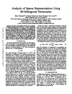
1, 2, · · · , T∗ }. Given a vector r on the N dimensional complex hypersphere, the SMDD algorithm find the closest Pk , k = 1, 2, · · · , T∗ to r. In other words, it minimizes ||r − ΠPk r||2 , where ΠPk is the projection operator onto Pk . Using this geometric interpretation, we will find a lower bound on the distortion as a function of sparsity and redundancy of any frame F . To this end, we define an L√ dimensional complex generalized cap of radius ρ around an L-dimensional plane Pk as GCL (ρ, Pk ) = {x ∈ SN : ||x − ΠPk x||2 ≤ ρ}

(21)

where SN is the N dimensional complex unit hypersphere {x ∈ CN : ||x||2 = 1}. If we are only interested in the radius of the generalized cap, but not the specific plane, we will use the notation GCL (ρ). In  order to calculate the  quantity of interest, 1 2 for √rN uniformly N Er min1≤k≤T∗ ||r − ΠPk r|| distributed on SN , we need to know the distribution of mink d2 (x, Pk ), where d2 (x, Pk ) , ||x − ΠPk x||2 and x is uniformly distributed on SN . Clearly, for any given x ∈ SN , we have P(min d2 (x, Pk ) ≤ η) k

√ = P(There exists a plane within distance η of x) = P(x is in the area covered by the generalized √ caps of radius η)   T∗ [ GCL (Pk , η) x =P x∈ k=1

Since T∗ ≤ T   T∗ [ P x∈ GCL (Pk , η)

Thus

(22)

k=1

P(min d2 (x, Pk ) ≤ η) ≤ T k

and

A(GCL (η)) , A(SN )

  A(GCL (η)) , 0 (23) P(min d2 (x, Pk ) ≥ η) ≥ max 1 − T k A(SN ) In order to bound

E(min d (x, Pk )) = k

Z

1 0

||U ∗ x − DU ∗ x||2 , and U ∗ x is just a unitary transformation of x that has the same uniform distribution as x. Let w be a vector uniformly distributed on the unit hypersphere. One way to generate w is to take a complex zeromean Gaussian vector z ∼ Nc (0, IN ), where IN is the identity z matrix, and let w = ||z|| [8] (Thm 1.5.6). Clearly w has the same distribution as U ∗ w, and thus ||w − ΠP w||2 has the same distribution as ||w − Dw||2 = |wL+1 |2 + · · · + |wN |2 . It is easy to see that

P(min d2 (x, Pk ) ≥ η)dη k

We will establish a lower bound on the right hand side of Inequality (23), by the value of η for which 0 =
estimating
1 − T A GCL (η) /A SN . Clearly ΠP satisfies: Π∗P = ΠP and Π2P = ΠP . It is wellknown that the projection matrix ΠP can be diagonalized as ΠP = U DU ∗ , where U is a unitary matrix and D is a diagonal matrix with 1’s as the first 1, 2, · · · , L and 0’s as the rest of N − L diagonal entries. Also we note that ||x − ΠP x||2 =

|zL+1 |2 + · · · + |zN |2 |z1 |2 + · · · + |zN |2

||w − Dw||2 =

where each zi ∼ Nc (0, 1) is a complex Gaussian random variable. It is well known [8] (Thm 1.5.7) that this fraction has β(N − L, L) type distribution. Thus Z ρ P(||w − Dw||2 ≤ ρ) = CN,N −L xN −L−1 (1 − x)L−1 dx 0

where CN,N −L =

Γ(N ) Γ(N −L)Γ(L) .

P(||w − Dw|| ≤ ρ) =

  T∗ X A(GCL (η)) P x ∈ GCL (Pk , η) ≤ T A(SN )

2

A Generalized Cap in RN with N = 3, L = 2

2

k=1

≤

Fig. 1.

But also

Z

GCL (ρ)


A GCL (ρ) 1
dw =
A SN A SN

Therefore for an L-dimensional generalized cap in CN we have
Z ρ A GCL (ρ) Γ(N )
= xN −L−1 (1 − x)L−1 dx N Γ(N − L)Γ(L) A S 0 (24) We now prove a number of technical lemmas. Lemma 3.1: Z ρ xN −L−1 (1 − x)L−1 dx ≤ 0 N −L−1 Z ρ x dx 1 + NL−1 0 −L−1 x Proof:  (1 − x)L−1 1 +

N −L−1 L−1 x ≤ N −L−1

e−(L−1)xe(L−1)x = 1

Hence we have (1 − x)L−1 ≤

1 1+


N −L−1 L−1 N −L−1 x

Substituting this to the integral gives the desired result.

6

DRAFT

Lemma 3.2: Let f (x) =

x , 1+ N L−1 −L−1 x

then f (x) attains its

maximum for x ∈ [0, ρ] at ρ. Proof: By direct computation, we have f ′ (x) =

1 (1 +

L−1 2 N −L−1 x)

Proof: The results for L = 0 and L = N are obvious. Thus without loss of generality, we can assume 1 ≤ L ≤ N − 1. Hence T > 1. For 1 ≤ L ≤ N − 2, we first claim that

for x ∈ [0, ρ]. Thus f (x) is an increasing continuous function that attains it maximum at ρ. We conclude from the above lemma that N −L−1 N −L−1  Z ρ x ρ dx ≤ 1 + N L−1 1 + NL−1 0 −L−1 x −L−1 ρ

Clearly, 2

Γ(N ) ≤ (N − 1)2(N −2)H Γ(N − L)Γ(L)

L−1 N −2

Proof:




By combining these results, we obtain the following bound:
L−1 A(GCL (ρ)) (N −2)H N −2 ≤ T (N − 1) 2 T A(SN )  N −L−1 ρ , Λ(ρ, N ) (25) 1 + NL−1 −L−1 ρ κc (N ) , T

(N − 1)

2

L−1 N −2

then




, (26)

Lemma 3.4: For any frame F of dimension N and size M over C, and for a sparse representation over F for x uniformly distributed on the unit hypersphere SN , with at most L = ǫN nonzero coefficients, we have 2 • For L = 0, P(mink d (x, Pk ) ≥ ρ) = 1 for any 0 ≤ ρ ≤ 1. • For 1 ≤ L ≤ N − 2, the equality Λ(ρ, N ) = 1 is attained at κc (N ) (27) ρ = ρ0 (N ) , 1 − NL−1 −L−1 κc (N ) −1

N −2

•

L−1 N −2

  NL−1 −L−1

 N −L−1 , N −2

−1

The claim is proved since T N −L−1 < 1, (N −1) N −L−1 ≤ 1,
N −2 L−1 N −L−1 ≤ 1. The value of ρ0 (N ) and the fact that and N −2 ρ0 (N ) ≥ 0 now follows from Equation (25). Since

T A GCL (ρ0 (N )) /A SN ≤ Λ(ρ0 (N ), N ) = 1,

we have A GCL (ρ0 (N )) /A SN ≤ 1 and thus ρ0 (N ) ≤ 1 as claimed. For L = N − 1, we directly calculate Z ρ A(GCL (ρ)) (N − 1)(1 − x)N −2 dx = 1 − (1 − ρ)N −1 = A(SN ) 0 Therefore T A(GCL (ρ))/A(SN ) becomes 1 at  1  1 N −1 ρ0 (N ) = 1 − 1 − T

We now prove the main result of this section. Theorem 3.5: For any frame F over C of dimension N , redundancy r − 1 = M/N − 1, for sparsity factor ǫ = L/ N , and for r uniformly √ distributed on the N -dimensional hypersphere of radius N , we have • For L = 0, we have D(F ) = 1. • For 1 ≤ L ≤ N − 2, we have  1  D(F ) = Er min ||r − ΠPk r||2 1≤k≤T N ρ0 (N )2 1 ≥ ρ0 (N ) − κc (N ) N − L where,

ρ0 (N ) =

L−1

κc (N ) , T N −L−1 (N − 1) N −L−1 2− N −L−1 H( N −2 ) •

=



−1 −1 L−1 κc (N ) = T N −L−1 (N − 1) N −L−1 N −L−1   L−1   L − 1 N −L−1 L−1 N −2 N −2

where −1




and 0 ≤ ρ0 (N ) ≤ 1.

We define −2 − NN −L−1 H

L−1 N −2

(28)

−1

(N − 1)! Γ(N ) = Γ(N − L)Γ(L) (N − L − 1)!(L − 1)!   N −2 = (N − 1) L−1
L−1 (N −2)H N −2 ≤ (N − 1)2

−1 N −L−1

−2 − NN −L−1 H

thus

Lemma 3.3:

−1 N −L−1

L−1 κc (N ) < 1 N −L−1

>0

and 0 ≤ ρ0 (N ) ≤ 1.

For L = N − 1, T A GCL (ρ) /A SN = 1 at  1  1 N −1 . ρ0 (N ) = 1 − 1 − T For L = N , P(mink d2 (x, Pk ) ≥ ρ) = 0 for any 0 < ρ ≤ 1.

1−

κc (N ) L−1 N −L−1 κc (N )

and −1

−1

N −2

L−1

κc (N ) = T N −L−1 (N − 1) N −L−1 2− N −L−1 H( N −2 ) . •

For L = N − 1,   1 Er min ||r − ΠPk r||2 D(F ) = 1≤k≤T N   1 1 N ≥ ρ0 (N ) − T ρ0 (N ) − + (1 − ρ0 (N )) N N

DRAFT

7

where

•

Also

 1  1 N −1 ρ0 (N ) = 1 − 1 − . T

g(y) = 

For L = N , we have D(F ) = 0.

Proof:√The results for L = 0 and L = N are obvious. Let x = r/ N , then Z 1 D(F ) = E(min d2 (x, Pk )) = P(min d2 (x, Pk ) ≥ η)dη k

k

0

≤

1 − κc (N ) NL−1 −L−1 y κc (N ) 1 − κc (N ) NL−1 −L−1

0

1

D(F ) ≥ ρ0 (N ) −

k

Combining the above and by applying Lemma (3.4), we have Z ρ0 (N ) (1 − Λ(η, N ))dη D(F ) ≥ 0

for 1 ≤ L ≤ N − 2 and  Z ρ0 (N )  A(GCL (η)) dη D(F ) ≥ 1−T A(SN ) 0

= ρ0 (N ) −

Z

1+

ρ0 (N )

L−1 N −L−1 η

L−1 N −2

L−1

T (N − 1)2(N −2)H N −2 0 N −L−1  η dη 1 + NL−1 −L−1 η

1

1

N −2

=

L−1 N −2




1 η κc (N ) 1 + N L−1 −L−1 η


(29)

η L−1 N −L−1 η

(30)

where κc (N ) is defined as in Equation (26). Clearly y ranges from 0 to 1 in this case. Also η=

(35)

We note that all the bounds attain values in [0, 1], since we have integrated a function that takes values in [0, 1] over a region [0, ρ0 (N )] ⊆ [0, 1]. Theorem 3.5 gives a fundamental limit on average distortion that any frame over C has to satisfy. We now fix r and ǫ and let N → ∞. The following asymptotic result follows: Corollary 3.6: For any frame F over C of dimension N , redundancy r−1 = M/N −1, for sparsity factor ǫ = L/N and for r uniformly distributed on the N -dimensional hypersphere √ of radius N , as N → ∞, we have D(F ) ≥

1+

ρ0 (N )2 1 κc (N ) N − L

and the result for 1 ≤ L ≤ N − 2. For L = N − 1,   Z 1 A(GCL (η)) D(F ) ≥ max 1 − T , 0 dη A(SN ) 0 Z ρ0 (N )   = 1 − T 1 − (1 − η)N −1 dη

We will next bound the last integral. Let y = T N −L−1 (N − 1) N −L−1 2 N −L−1 H

(34)

and the result follows easily by direct integration.

N −L−1 # dη




(33)

0

0

η

ρ0 (N )2 κc (N )

which gives us

P(min d2 (x, Pk ) ≥ η) ≥ max(1 − Λ(η, N ), 0)



2 =

ρ0 (N )2 N −L−1 ρ0 (N )2 1 y dy = κc (N ) κc (N ) N − L

By applying Inequality (25), we have

for L = N − 1. Thus for 1 ≤ L ≤ N − 2 Z ρ0 (N ) " 1 − T (N − 1) 2(N −2)H D(F ) ≥

2

since g ′ (y) > 0 for y ∈ [0, 1]. Thus the last integral in Equation (29) is bounded above by Z

and we have previously proved that   A(GCL (η)) P(min d2 (x, Pk ) ≥ η) ≥ max 1 − T , 0 . k A(SN )

κc (N )

κc (N )y 1 − yκc (N ) N L−1 −L−1

(31)

Since by Equation (28), κc (N ) N L−1 −L−1 < 1, and 0 ≤ y ≤ 1, the denominator of the above is not equal to 0 within the region of integration. Now we note that κc (N ) dη =  2 dy , g(y)dy. L−1 1 − yκc (N ) N −L−1

(32)

κ0 (1 − ǫ) 1 − ǫκ0

(36)

where
ǫ r ǫ (37) κ0 = 2− 1−ǫ H r ǫ 1−ǫ Proof: The result follows by replacing M = rN and L = ǫN in the statement of Theorem 3.5 and using

1 rN H rǫ rN H rǫ 2 ≤T ≤2 M +1 and lim κc (N ) = κ0 (1 − ǫ).

N →∞

It is noteworthy that the above asymptotic corollary can be proven by combining a result of Sakrison [10] with the proof method of [6], although the setting and the topic of our paper is very different from these papers.

8

DRAFT

IV. C ONCLUSION In this paper, we considered approximations of signals by the elements of a frame in a complex vector space of dimension N . We formulated both the noiseless and the noisy sparse representation problems. For the noiseless representation problem, it is known in advance that the signal r has a sparse representation in terms of the elements of the frame F . In this case, the goal is to find a solution to the sparse representation problem in real time. We provided a solution to this problem, by explicitly constructing a frame, which we referred to as the Vandermonde frame, for which the noiseless sparse representation problem can be solved uniquely using O(N 2 ) operations, as long as the number of non-zero coefficients in the sparse representation of r is ǫN for some 0 ≤ ǫ ≤ 0.5. This result improves on a result by Candes and Tao [3]. We also showed that ǫ ≤ 0.5 cannot be relaxed without violating uniqueness. For the noisy sparse representation problem, we considered the case when the signal r cannot be represented in terms of the elements of the frame F in a sparse manner and noted that any such representation suffers from distortion. In this case, we established a lower bound on the trade-off between sparsity, distortion and redundancy. Our future research will focus on constructing frames for which not only these trade-offs can be achieved, but also the underlying sparse representations can be found in real time. ACKNOWLEDGMENT The authors would like to thank Robert Calderbank, Ingrid Daubechies and David L. Donoho for many insightful discussions. R EFERENCES [1] E. J. Candes and J. Romberg, “Practical signal recovery from random projections”, preprint. [2] E. J. Candes, J. Romberg, and T. Tao, “Stable signal recovery for incomplete and inaccurate measurements”, preprint. [3] E. J. Candes and T. Tao, “Decoding by Linear Programming”, IEEE Trans. on Inf. Theory, vol. 51, no. 12, pp. 4203-4215, Dec. 2005. [4] S. S. Chen, D. L. Donoho, and M. A. Saunder “Atomic decomposition by basis pursuit”, SIAM J. Sci. Comput., vol. 20, no. 1, pp. 33-61, July 2003. [5] D. L. Donoho, M. Elad, and V. N. Temlyakov, “Stable recovery of sparse overcomplete representations in the presence of noise”, IEEE Trans. on Inf. Theory, vol. 52, no. 1, pp. 6-18, Jan. 2006. [6] A. K. Fletcher, S. Rangan, V. K. Goyal, and K. Ramchadran, “Denoising by Sparse Approximation: Error Bounds Based on Rate-Distortion Theory”, EURASIP Journal on Applied Signal Processing, Vol. 2006, Article ID 26318, pp. 1 - 19. [7] F. J. MacWilliams and N. J. A. Sloane, The Theory of Error Correcting Codes, Ninth Edition, Elsevier Scince Publishers, Amsterdam, 1996. [8] R. J. Muirhead, Aspects of Multivariate Statistical Theory, John Wiley & Sons, 1982. [9] M. Rudelson and R. Vershynin, “Geometric approach to error correcting codes and reconstruction of signals”, preprint [10] D. J. Sakrison, “A Geometric Treatment of the Source Encoding of a Gaussian Random Variable”, IEEE Trans. on Inf. Theory, vol. 14, no. 3, pp. 481 - 486, May 1968. [11] M. Sudan, “Decoding of Reed Solomon codes beyond the errorcorrection bound”, Proceedings of the 37th Annual Symposium on Foundations of Computer Science, pp. 164-172. [12] J. A. Tropp, “Topics in Sparse Approximation”, Ph.D. dissertation, Computational and Applied Mathematics, UT-Austin, August 2004.

[13] J. A. Tropp, “Greed is Good: Algorithmic Results for Sparse Approximation”, IEEE Trans. on Inf. Theory, vol. 50, no. 10, pp. 2231-2242, Oct. 2004. [14] J. A. Tropp and A. C. Gilbert, “Signal recovery from partial information via Orthogonal Matching Pursuit”, preprint.