approach applies a 3D registration technique based on point- ... Especially in these domains, ... One approach that deals with real objects was presented.
Learning the Elasticity Parameters of Deformable Objects with a Manipulation Robot Barbara Frank
R¨udiger Schmedding
Cyrill Stachniss
Abstract— In this paper, we consider the problem of determining the elasticity properties of deformable objects with a mobile manipulator equipped with a force sensor.b We learn the parameters by establishing a relation between the applied forces and the corresponding surface deformations. To determine the parameters, we minimize the difference between the observed surface of an object that is deformed by a real manipulator and the deformed surface obtained with a deformation simulator based on finite element methods. To establish the correspondences between the surfaces, our approach applies a 3D registration technique based on pointclouds which is used as the basis for comparing the results of the simulation system with the observations of the real deformations. As we demonstrate in real-world experiments, our system is able to estimate appropriate parameters that can be used to predict future deformations. This information can directly be incorporated into motion planning approaches that are designed for robots operating with deformable objects.
Matthias Teschner
Wolfram Burgard
Fig. 1. Deformation of an object in reality (left) and the 3D perception of the robot (right).
A lot of effort has been invested into the simulation of deformations and the generation of realistic deformable models. There exists a variety of relevant applications in computer graphics, robotics [21], virtual reality, games, movies, and medical simulation [16, 7, 19]. As we demonstrated in the past [10, 11], robots that are able to deal with deformable objects in their environment can greatly improve their navigation skills in the real world, especially in domestic settings. Planning techniques as well as most other applications considering deformations require an appropriate model including reasonable elasticity parameters of objects in the scene. In practice, the parameters are typically adjusted manually. Thereby, the parameters are usually modified until the simulation looks visually plausible. This might be applicable for computer games or movies, but does not necessarily lead to a physically realistic computation of the involved forces. These forces, however, need to be known accurately for navigation or manipulation in the presence of deformable objects. For example, whenever robots interact with realworld objects, only limited forces should be applied to them. This is of utmost importance in medical applications but also in domestic settings, for example when robots have to manipulate plants or clothes. Especially in these domains, robots need exact knowledge about the parameters of the deformation process.
Generating realistic models of deformable objects not only involves observing and reconstructing the three-dimensional surface of an object. Physical interaction with the object under consideration is required to learn about its behavior when exposed to external forces. Therefore, we equipped our robot with a force sensor at the end of the manipulator. This allows the robot to interact with objects and to measure the forces exerted on them. The robot can additionally perceive the objects with a range camera. To reduce the effect of occlusions during the deformation, our robot uses a rigid stick to deform the object (see Figure 1). Based on the observed deformations and forces, our approach seeks to estimate the elasticity parameters of the object. This is done by simulating the object and the applied forces. In our approach, we consider homogeneous and isotropic materials and use a linear finite element model to compute deformations. An error minimization approach is applied to iteratively update the deformation parameters so that the difference between the real object under deformation and the simulation is minimized. As we will demonstrate in the experimental section of this paper, our approach is able to find the elasticity parameters that enable our robot to accurately predict the deformation of real-world objects. This paper is organized as follows. After discussing related work in the following section, we present in Section III an overview of our system for data acquisition and parameter estimation. In Section IV, we present the deformation simulation before we describe how to acquire data of deformed objects with a real robot in Section V. Section VI then contains our approach to parameter estimation. Finally, in Section VII, we present experimental results.
All authors are with the Department of Computer Science, University of Freiburg, 79110 Freiburg, Germany. {bfrank,stachnis,schmedd,burgard,teschner}@informatik.uni-freiburg.de This work has partly been supported by the German Research Foundation (DFG) under contract number SFB/TR-8.
Deformable modeling and parameter estimation are active areas of research. To represent non-rigid objects and to simulate deformations, mass-spring systems have been frequently
I. I NTRODUCTION
II. R ELATED W ORK
used. They are easy to implement and can be simulated efficiently [24, 8]. While such models are able to handle large deformations, their major drawback is the tedious modeling as there is no intuitive relation between spring constants and physical material properties in general [18]. Finite element methods (FEMs) reflect physical properties of the objects in a more natural way [1]. This allows for more intuitive modeling since they require only a small number of parameters. The disadvantage of FEMs lies in the computational resources required to calculate deformations. A computationally more efficient approach, which we also use in our current system, is the co-rotational finite element approach [12, 17] that avoids nonlinear computations. There exist some approaches to determine the physical parameters of models. Bianchi et al. [4] learn the stiffness constants of mass-spring models by using a genetic algorithm and comparing it to a FEM reference model. The identification of mass-spring parameters is also discussed in the work of Lloyd et al. [15]. They derive an analytical formulation for the spring parameters from the linear finite element model for different mesh topologies. Another approach that estimates the stiffness properties of mass-spring models was proposed by Burion et al. [6]. They use a particle filter to obtain a posterior distribution over the stiffness parameters and evaluate the particles by comparing simulated and observed deformations. In contrast to our work, they do not compare the deformed surfaces but the measured forces in the single nodes of the object. Furthermore, we do not only work on simulated data. Becker et al. [2] presented an approach for the estimation of elasticity parameters for the finite element method using Quadratic Programming. However, they also work on simulated data only. One approach that deals with real objects was presented by Lang et al. [14]. They describe a deformable model as a discrete boundary value problem and estimate Greens’ functions from measured forces and displacements. They formulate the estimation of the deformation matrix as a linear estimation problem. Fong [9] presents a system to measure deformations of elastic objects using a structuredlight camera and a force-sensor. They extract force-fields for different contact points and displacements on the objects. For haptic rendering of unseen contact points the forces are interpolated using radial basis functions. In a similar way, Bickel et al. [5] present a data-driven representation of heterogeneous and non-linear material by fitting radial basis functions to different measured force-displacement samples. They, however, use an underlying linear finite element model, similar to our approach, to model the different homogeneous parts of objects. In contrast to most of the previous approaches our method has been realized on a real mobile manipulation robot and deals with real data. In our setup, the mobile manipulation robot furthermore carries its sensors on-board and thus is the basis for fully autonomous exploration. Furthermore, the resulting models can directly be used for simulations, which have been shown to be relevant to robot navigation in environments containing deformable objects [10, 11].
III. S UMMARY OF OUR A PPROACH Our approach to determining physical deformation models consists of two main steps: • •
data acquisition with a manipulator (Section V), and parameter estimation via simulation and error minimization (Section VI).
In the data acquisition process, our robot interacts with an object and measures the forces it exerts on the object. Additionally, it observes the surface of the undeformed and deformed object with a depth camera. This allows us to estimate a relationship between the displacement of the surface points, the applied forces and the physical elasticity parameters. IV. D EFORMATION S IMULATION The key idea of our elasticity parameter estimation approach is to modify the parameters of a realistic simulation system until the deformations obtained in simulation approximate the ones measured on the real object. Thereby the force exerted on the simulated object is approximately identical to the one applied in the real world. Additionally, the points where the forces are applied correspond to each other. In this section, we describe our simulation environment that is based on finite element methods and is used to deform the virtual object. A. Modeling Objects using Tetrahedral Meshes To simulate the deformations of the object, our system requires a volumetric model of the object. Such models can be obtained in advance by registering multiple 3D point clouds obtained with a range scanner (see Section V-B). From these point clouds, we then generate a triangular surface mesh which in turn is used to determine the volumetric tetrahedral mesh needed to calculate the internal forces based on force-displacement-relations. To establish this tetrahedral mesh, we employ the meshing approach by Spillmann et al. [23]. This approach is particularly suited for real-world data, as it can handle unorientable, non-manifold, and even incomplete data. In this approach, one first computes a signed distance field where voxels having a negative sign represent the volume of the object. In a second step, one divides the spatial domain by a uniform axis-aligned grid. We discard all cells of this grid that do not contain any voxel with negative sign. The remaining cells are an approximation of the object’s volume, whose quality is given by the grid resolution. We divide these cells into five tetrahedrons each. In a post-processing step, we smooth the tetrahedrons to align with the given surface mesh. In our simulator, we perform all deformation computations based on the tetrahedral mesh. The coupling of the surface mesh to the tetrahedral mesh guarantees that the surface mesh is also deformed. This allows us to compare it to the scanned surface mesh of the real-world object.
B. Elasticity Parameters In our approach, we assume a linear and isotropic and homogeneous deformation model. The physical elasticity properties of such isotropic and homogeneous materials can mainly be described by two parameters, the Young modulus and the Poisson ratio. One can visualize the Young modulus as a measure for the force that is needed to enlarge respectively compress an object by some fixed amount. The Poisson ratio can be seen as a measure for the change of the thickness of the object’s material perpendicular to the direction of the enlargement respectively the compression. If a force F is applied to a bar of cross-section area A and length L, the bar enlarges by an amount ∆l which is 1 . This can be written as proportional to F, L and A ∆l
=
1 LF , E A
(1)
where the constant of proportionality E is called the Young modulus. Its unit is force per area and it is frequently N specified in mm 2. In contrast to the Young modulus, the Poisson ratio is related to the contraction perpendicular to the direction of the force. In our example, the force F causes a contraction ∆d perpendicular to the direction of the force. Let d be the thickness of the bar, ∆d d the relative change of its thickness, ∆l and L the relative change of its length. Then, the ratio of the relative changes given by ν
=
L∆d d∆l
(2)
is called the Poisson ratio ν, which is dimensionless. While there is no theoretical upper bound for the Young modulus, one can show that for real objects, the Poisson ratio lies within the range of 0 and 0.5. A Poisson ratio of 0.5 would imply perfect volume conservation, while a Poisson ratio of 0 would imply no volume conservation at all. C. Deformation Model Although our parameter estimation approach is independent of the underlying deformation model, we briefly introduce the basics of finite element methods used in our simulator. To simulate the dynamic behavior of an object and the reaction to external forces, we have to compute the internal forces that act inside the object depending on the current deformation. These forces are computed using a force-displacement-relation that is derived from the underlying deformation model. The basic idea of finite elements is to divide an object into smaller elements and to establish the force-displacementrelations on these small elements. In our case, these elements are the tetrahedrons mentioned above. This allows us to assume constant stress over an element, which results in a linear force-displacement-relation. Putting all these relations together, one can establish the so-called stiffness matrix K = K(E, ν) that depends on the Young modulus E and the Poisson ratio ν. For n being the number of vertices of
an object, the dimension of K is 3n × 3n. The global forcedisplacement relation then becomes f = Kq,
(3)
3n
where f ∈ R is the internal force induced by the displacement q ∈ R3n of the vertices of the tetrahedral mesh. The stiffness matrix allows us to compute the internal forces resulting from a deformation. To be able to establish the inverse relation q = K−1 f , (4) we have to consider some essential properties of K, as K is not invertible in general. However, it can be shown that K is invertible for a subspace, and that this subspace of deformations and forces contains exactly those forces and displacements which are interesting for the estimation process. First, it can be easily shown that K is symmetric and, hence, it is diagonalizable. Moreover, it can be shown that exactly six eigenvalues are equal to zero, and further, that these eigenvalues correspond exactly to the eigenvectors that represent the three possible directions of translation and three dimensions of infinitesimal rotations. That means, that exactly the forces that cause translations and infinitesimal rotations do not lie in the image space of K. Hence, all remaining forces have an inverse image q with Kq = f . If we additionally claim that q is orthogonal to the eigenvectors of translation and rotation, the inverse image is unique. Thus, restricting ourselves to forces that do neither cause translations nor rotations, we are able to write the inverse relationship q = K−1 f . Restricting to those forces having an inverse image is exactly what we do in the real world experiments: In order to ensure that the robot deforms an object and the force it measures corresponds to the deformation, we fix the object under consideration. Furthermore, by applying a registration of the surfaces, we eliminate the effects of small translations and rotations in the measured displacement. Although we do not need the inverse for the computation, but only as a theoretical argument, we show how K−1 could be computed. First, we compute the diagonal matrix DK = QKQT , where Q is an orthogonal matrix. Then, we take the inverse of all non-zero eigenvalues and do not change the zero eigenvalues which results in D−1 K , restricted to those vectors in the image space having an inverse image. Then, the inverse K−1 is given as QT D−1 K Q, also restricted to those vectors having an inverse image. V. DATA ACQUISITION In this section, we present our robotic system that is used for the acquisition of deformable models. A. Technical Details Our system for acquiring real data consists of a mobile platform with a 7-DoF manipulator that is equipped with a force-torque sensor and a depth camera (see Figure 2 (a)). This setup allows us to observe objects from different view points, to deform them and to measure the corresponding deformation forces in a flexible way.
(a)
(b)
(c)
(d)
Fig. 2. Object reconstruction: The robot observing a deformable teddy bear (a), a point cloud obtained with the time-of-flight camera (b), surface mesh constructed from four different point clouds (c), and the tetrahedral mesh computed from the surface mesh (d).
The manipulator consists of five Schunk Powercube modules and a 2-DoF hand. These modules have a high repeat accuracy of 0.02◦ and therefore allow for an accurate estimation of the robot’s position. We measure the deformation forces with a Schunk-FTCL-050 force-torque sensor integrated into the hand. This sensor is able to measure forces up to 300 N and torques up to 7 Nm in all three degrees of freedom. To perceive the object, we employ either a Bumblebee stereo camera or a PMD-[vision]-O3 timeof-flight camera, which is attached to the gripper of the manipulator. Both cameras can be easily exchanged, and we experimented with different depth sensors that both have different drawbacks and advantages: the stereo camera has a higher resolution, a bigger field of view, and gives good results with textured objects. However, for uniformly colored objects, the depth data is unsatisfactory. For such objects, we used a time-of-flight camera. This type of camera has a rather limited field of view, and the measurements are affected by different sources of noise, for instance the illumination, the color of objects, and the distance to the object. B. Geometrical Models for Simulation For the simulation of deformations, a volumetric model is required (see Section IV-A). Such a model can be computed from a surface mesh of the object. We can obtain such a surface mesh by exploring the space and by scanning the object from different view points as described in a prior work [25]. These point clouds are then registered into a consistent model (see Figure 2). A more efficient way is to first take an observation of an undeformed object and complete it heuristically by assuming a planar surface on the backside, which can be extracted for instance from the table or the wall that limit the maximum extent of the object. This allows us to immediately start manipulating the object and estimating its deformation parameters. Our experiments show that a complete model is not needed to estimate the deformation parameters – a partial model is sufficient. C. Deformation of Objects To actually interact with the object, the robot uses its manipulator to apply a force to the object. Whenever a force is applied, we measure the surface points of the deformed object to relate the forces to deformations. One practical problem occurring at this point is that a robot that deforms
an object obviously occludes the deformed object part and that the manipulator always is part of the observation. To limit the occlusions introduced by the manipulator deforming the object, we use a thin wooden stick attached to the end-effector. This yields observations of the surface with minimal occlusions. We use the model of the robot’s body to label parts of the image as invalid where the measurements correspond to the robot, and not to the object. Furthermore, in order to ensure, that the object is deformed and not moved by the robot, we assume that it is lying on a table or fixed by a wall. In our current implementation, the robot approaches the object, and step by step, increases the force, until a maximum force of 50 N is applied or the end-effector moved for more than 10 cm. In this way, we obtain a set of force measurements ztf ∈ R3 in combination with corresponding surface meshes zts ∈ R3n for every point in time t. VI. PARAMETER E STIMATION In this section, we explain our approach to estimate the Young modulus E and the Poisson ratio ν for real objects based on observations of our robot. The key idea of our approach is to apply a gradient–descent based error minimization approach to minimize the difference between the real deformation and the simulated one given the elasticity parameters. A. Error Function To apply gradient descent, we need to define an appropriate error function, which in our case should reflect the difference between the measured and the simulated surface, since the surface can be observed by the robot. To compute this difference, we first align the deformed surfaces with a registration procedure and then measure the remaining difference. The task of registration algorithms is to align multiple overlapping scans of the same object, i.e., to compute a translation and a rotation that align the surfaces correctly. In our approach, we apply the ICP-algorithm by Besl and McKay [3], with some extensions similar to the ideas given by Pulli [20] and Rusinkiewicz [22]. For known correspondences, the transformation can be computed directly [13]. Since the correspondences are not known in general, the ICP algorithm determines some correspondences, e. g. by using a nearest-neighbor data association, computes a transformation that aligns the scans for these correspondences, and then determines new correspondences to compute a new relative position. Typically, this procedure converges to a minimum and yields an accurate alignment if a proper initial configuration is chosen. In our system, we can easily derive a good initial alignment from the position of the manipulator to which the camera is attached. The quality of the initial alignment mainly depends on the quality of the encoders in the manipulator. These encoders are typically accurate and for our robot, the error is around 0.02 degrees per joint and thus sufficient to allow the ICP algorithm to converge to an
accurate alignment. After applying ICP, we can define the error function between a model M and the measured surface z s as Err(E, ν)
=
dist(simulate(E, ν, M, ztf , pt ), zts ), (5)
with dist(Mdef , z s )
=
X i∈z s
min ||i − j||2 ,
j∈Mdef
(6)
where i and j refer to the points from the observed and the simulated surface, respectively.
(a)
(b)
2
After defining the error function above, we can apply gradient descent to seek for a Young modulus E and Poisson ratio ν that minimize the error. Algorithm 1 summarizes the main routine. The variable M refers to the undeformed object model which is generated from a first observation taken before the deformation starts. This model is the basis for all simulations. Line 3 of the algorithm requires to compute the partial derivative of the error function. Since the error function involves the simulation approach explained above, the derivatives cannot be computed easily. Thus, we approximate this term numerically: A sequence of deformation simulations is carried out by applying the measured force and by varying the E and ν locally. In the remainder of this section, we show that the gradient descent-based error minimization is well suited for this problem given a good initial guess. First, we show that parameters close to the correct ones result in a smaller difference in the displacement obtained in simulation and in reality than parameters far from the solution. Therefore, we relate the deviation between the correct and the estimated parameters to the deviation between the displacement in reality qr and the displacement in simulation qe using the force-displacement-relation of the finite element method:
0
= =
F F
(d)
RMSE (mm)
B. Gradient Descent for Parameter Estimation
Ke q e Kr q r
(c)
Fig. 3. Registration results for simulated data: the error decreases if the N estimated parameters converge to the correct parameters E = 1000 mm 2, N ν = 0.3. The estimated parameters are (a) E = 3000 mm , ν = 0.3, 2 N N (b) E = 2000 mm 2 , ν = 0.3, (c) E = 1300 mm2 , ν = 0.3 and (d) N E = 1000 mm 2 , ν = 0.3.
1
(7) (8)
0.4 1200 0.3 Poisson ratio ν
1000 0.2
800
Young modulus E
Fig. 4. Convexity of the error function. The “correct” values are given N by E = 1000 mm 2 and ν = 0.3. Varying values for E and ν result in a registration error which gets bigger the farther the estimated parameters are away from the correct ones.
By inverting Ke and Kr , we obtain qe qr
= =
K−1 e F K−1 r F.
Then, the quadratic deviation can be written as
2 2 −1
kqr − qe k = (K−1 r − Ke )F
(9) (10)
(11)
As F is fixed in Eq. (11), we see that smaller deviations in measured and simulated displacements directly correspond to smaller deviations between the estimated and the real stiffness matrix. This makes it reasonable to compare simulated and measured displacements in order to estimate these parameters. VII. E XPERIMENTAL E VALUATION The approach above has been implemented and evaluated in several experiments using real and simulated data.
Algorithm 1 Iterative parameter estimation
A. Simulation Experiment
Require: Object model M , observations ztf , zts , contact point pt , 1: Initialize (E0 , ν0 ), i=1 2: loop 3: (Ei , νi )T = (Ei−1 , νi−1 )T − λ∇Err(Ei−1 , νi−1 ) 4: Mdef = simulate(Ei , νi , M, ztf , pt ) 5: err = dist(Mdef , zts ) 6: if err < ǫ then 7: return (Ei , νi ) 8: end if 9: i++ 10: end loop
The first experiment carried out in simulation is designed to show that our approach works under comparably welldefined conditions and is able to find the correct elasticity parameters. In this experiment, we used a cow as a complex N geometric object with a Young modulus of 1000 mm 2 and a Poisson ratio of 0.3. We executed our gradient descent-based estimation procedure after we deformed the cow with a given constant force. Our method changes the elasticity parameters in simulation and performs a registration step to match the model with unknown parameters against the model with known ones. Figure 3 illustrates the results in terms of the model matchings for different parameter estimates. The red and the
50
RMSE (dm)
30 20
0.07 0.06 0.05
10
0.04
0 0
20
40
60
80
0
100
(a) Young modulus E (N/dm2)
100
200
300
Young modulus (N/dm2)
Distance (mm)
(b)
Fig. 7. The tetrahedral model of the inflatable balloon: undeformed (left) and deformed with optimized parameters (right).
350 300 250 200 150 100 2
4
6 8 10 Experiment
12 mean
(c) Fig. 5. Experiment with a foam cube: force-distance curve derived from the manipulator movement (a), the error function for one example estimation experiment (b), and the estimated young modulus for different force-deformation samples (c).
Fig. 6. Registration result of the deformed cube. Scan of the real cube (left), simulation result (middle), and matching between the scanned and the simulated model under deformation (right).
yellow areas correspond to the different models. In the left image, a clear mismatch between the objects can be observed since a correct alignment is impossible due to the different object deformations. As the Young modulus approaches the N correct value of 1000 mm 2 (from left to right), the two models become more similar until the optimal parameter set is found (right image). Figure 4 illustrates the error surface for this experiment. B. Real World Experiments We tested our parameter estimation approach on different real-world objects, namely a foam cube, an inflatable balloon and a plush teddy bear. 1) Foam cube: In the first experiment, we determined the elasticity parameters of a foam cube with an edge length of 15 cm. The robot deforms the object in the center. The force-vs-distance curve of this experiment is shown in Figure 5 (a). In this experiment, we used the PMD timeof-flight camera. The robot moved for 9 cm and collected a force measurement and a surface scan every 1 cm. As can be seen in that curve, the deformation behavior of the cube is approximately linear, except in the beginning, where slippage of the probe tip occurred. This shows that our material assumptions are reasonable. We evaluated the error function for a uniform sampling of elasticity parameters in
Young modulus E (N/dm2)
Force (N)
model undeformed ν = 0.1 ν = 0.2 ν = 0.3 ν = 0.4
0.08
40
140 120 100 80 60 40 20 0 1
2
3
4
5
6
7
mean
Experiment
Fig. 8. Learning the deformation parameters of the inflatable balloon. Shown are results for different force-deformation samples.
order to investigate, whether it contains local minima. This is illustrated in Figure 5 (b). The error function is very high if the simulated object is too deformable and the Young modulus is too small, respectively, and slowly converges to the error of the undeformed mesh, as the object becomes stiffer with increasing young modulus. Furthermore, we note, that the Young modulus has a substantially larger influence on the error function than the Poisson ratio. The plot in Figure 5 (c) illustrates the learned Young modulus for the different force-deformation samples. It shows, that the variance of our learning method is rather low among the different runs. Figure 6 shows a comparison between the scanned and the simulated deformation for one of the experiments in Figure 5 (c). 2) Inflatable balloon: In a second experiment, we evaluated our gradient-descent based parameter estimation with the inflatable balloon that is shown in Figure 1. In this experiment, we used the Bumblebee stereo camera. First, a model of the undeformed object is constructed on the fly for the simulation system, as shown in Figure 7. Second, the ICP algorithm is used to obtain the alignment of the deformed model with the observation of the deformed object. Then, given the alignment, the error function can be computed. Furthermore, we repeated the experiment by applying different forces to the object to evaluate the robustness of the parameter estimation. We deformed the ball with seven substantially different forces and obtained seven different surface scans. The resulting estimate for the young modulus is shown in Figure 8. We can see that the estimation converges to similar values for the young modulus, indicating a homogeneous deformation behavior of the object. The simulations were carried out on a model that consists of 815 tetrahedrons. The average run-time for computing the optimal parameters per force-displacement sample was 192.5 seconds, on average 7 iterations of deformation simulations with different parame-
Young modulus E (N/dm2)
back
150
R EFERENCES
belly 100
head
50 0 1
2
3
4
5
6
mean
Experiment
Fig. 9. Parameter estimation results for deformation experiments with different body parts of the teddy bear. In each experiment, the average over different force-displacement samples was computed.
Fig. 10.
Comparison of the real deformation and the deformed model.
ters were needed before the parameter estimation converged. 3) Plush teddy: In order to evaluate the robustness of our parameter estimation, we furthermore deformed the plush teddy bear from Figure 2 at different body parts, e. g. the head, the belly, and the back, and analyzed the results of our parameter estimation approach. The results are summarized in Figure 9. In each experiment, the parameters were determined as the average over seven different forcedisplacement samples. Additionally, the mean over the six different experiments is shown. The variance among the different experiments is higher than the variance among different force-deformation samples for the same location, which suggests, that the assumption of homogeneous material is not valid in this case. Finally, Figure 10 illustrates in a comparison of the real and the simulated deformation that the estimated parameters still lead to plausible deformations. VIII. C ONCLUSIONS In this paper, we presented an approach for estimating the elasticity parameters of homogeneous isotropic deformable objects. These parameters are relevant for robots that need to estimate deformations of objects in their environment depending on the forces applied to them. Our approach uses a mobile robot that is equipped with a manipulator, a force sensor, and a depth camera. It applies a deformation force to an object and records the resulting force-displacement relation with the force sensor and the depth camera. Based on a gradient descent-based error minimization approach carried out within a realistic finite element-based simulation system, the robot can determine the elasticity parameters that best explain the real deformations. As we showed in our experiments, we are able to estimate the parameters of real objects in a robust manner.
[1] K.-J. Bathe. Finite Element Procedures. Prentice Hall, 2 edition, 1995. [2] M. Becker and M. Teschner. Robust and Efficient Estimation of Elasticity Parameters Using the Linear Finite Element Method. In Proc. of Simulation and Visualization, 2007. [3] P. Besl and N. McKay. A Method for Registration of 3-D Shapes. IEEE Transactions on Pattern Analysis and Machine Intelligence, 14(2):239–256, 1992. [4] G. Bianchi, B. Solenthaler, G. Sz´ekely, and M. Harders. Simultaneous Topology and Stiffness Identification for Mass-Spring Models based on FEM Reference Deformations. In Medical Image Computing and Computer-Assisted Intervention (MICCAI), 2004. [5] B. Bickel, M. Baecher, M. Otaduy, W. Matusik, H. Pfister, and M. Gross. Capture and Modeling of Non-Linear Heterogeneous Soft Tissue. Proc. of ACM SIGGRAPH, 28(3):1081–1094, 2009. [6] S. Burion, F. Conti, A. Petrovskaya, C. Baur, and O. Khatib. Identifying Physical Properties of Deformable Objects by Using Particle Filters. In Proc. of the Int. Conf. on Robotics & Automation (ICRA), 2008. [7] D. Chen and D. Zeltzer. Pump it up: Computer Animation of a Biomechanically Based Model of Muscle Using the Finite Element Method. In Proc. of ACM SIGGRAPH, 1992. [8] F. Conti, O. Khatib, and C. Baur. Interactive Rendering of Deformable Objects based on a Filling Sphere Modelling Approach. In Proc. of the Int. Conf. on Robotics & Automation (ICRA), 2003. [9] P. Fong. Sensing, Acquisition, and Interactive Playback of Data-based Models for Elastic Deformable Objects. Int. Journal of Robotics Research, 28:630–655, 2009. [10] B. Frank, M. Becker, C. Stachniss, M. Teschner, and W. Burgard. Efficient Path Planning for Mobile Robots in Environments with Deformable Objects. In Proc. of the Int. Conf. on Robotics & Automation (ICRA), 2008. [11] B. Frank, C. Stachniss, R. Schmedding, M. Teschner, and W. Burgard. Real-world Robot Navigation amongst Deformable Obstacles. In Proc. of the Int. Conf. on Robotics & Automation (ICRA), 2009. [12] M. Hauth and W. Strasser. Corotational Simulation of Deformable Solids. In Proc. of WSCG, 2004. [13] B. Horn. Closed-Form Solution of Absolute Orientation Using Unit Quaternions. J. Opt. Soc. Amer. A, 4(4):629–642, 1987. [14] J. Lang, D. Pai, and R. Woodham. Robotic Acquisition of Deformable Models. In Proc. of the Int. Conf. on Robotics & Automation (ICRA), 2002. [15] B. Lloyd, G. Szekely, and M. Harders. Identification of Spring Parameters for Deformable Object Simulation. IEEE Trans. on Visualization and Computer Graphics, 13(5):1081–1094, 2007. [16] M. Metzger, M. Gissler, M. Asal, and M. Teschner. Simultaneous Cutting of Coupled Tetrahedral and Triangulated Meshes and its Application in Orbital Reconstruction. Int. Journal of Computer Assisted Radiology and Surgery, 4(5):409–416, 2009. [17] M. Mueller and M. Gross. Interactive Virtual Materials. In Graphics Interface, 2004. [18] A. Nealen, M. Mueller, R. Keiser, E. Boxerman, and M. Carlson. Physically Based Deformable Models in Computer Graphics. Computer Graphics Forum, 25(4):809–836, 2006. [19] G. Picinbono, H. Delingette, and N. Ayache. Non-linear and Anisotropic Elastic Soft Tissue Models for Medical Simulation. In Proc. of the Int. Conf. on Robotics & Automation (ICRA), 2001. [20] K. Pulli. Multiview Registration for Large Data Sets. In Proc. of the Int. Conf. on 3D Digital Imaging and Modeling (3DIM), 1999. [21] S. Rodr´ıguez, J.-M. Lien, and N. Amato. Planning Motion in Completely Deformable Environments. In Proc. of the Int. Conf. on Robotics & Automation (ICRA), 2006. [22] S. Rusinkiewicz and M. Levoy. Efficient Variants of the ICP Algorithm. In Proc. of the Int. Conf. on 3D Digital Imaging and Modeling (3DIM), 2001. [23] J. Spillmann, M. Wagner, and M. Teschner. Robust Tetrahedral Meshing of Triangle Soups. In Proc. Vision, Modeling, Visualization (VMV), 2006. [24] M. Teschner, B. Heidelberger, M. Mueller, and M. Gross. A Versatile and Robust Model for Geometrically Complex Deformable Solids. In Proc. of Computer Graphics International, 2004. [25] R. Triebel, B. Frank, J. Meyer, and W. Burgard. First Steps towards a Robotic System for Flexible Volumetric Mapping of Indoor Environments. In Proc. of the IFAC/EURON Symposium on Intelligent Autonomous Vehicles (IAV), 2004.