changed (e.g. redirected upwards) and the gaze contact can be established. ... of methods offers a mixed software/hardware solution and proceed in two steps. First .... nally consider a bounding box B having the same center as B and having ...
Learning To Look Up: Realtime Monocular Gaze Correction Using Machine Learning Daniil Kononenko Victor Lempitsky Skolkovo Institute of Science and Technology (Skoltech) Novaya Street 100, Skolkovo, Moscow Region, Russia {daniil.kononenko,lempitsky}@skoltech.ru
Abstract
Most successful solutions to gaze correction have been so far relying on additional hardware such as semitransparent mirrors/screens [16, 12], stereocameras [23, 5], or RGB-D cameras [26, 14]. Because of the extra hardware dependence, such solutions mostly remain within the realm of high-end conferencing systems and/or research prototypes. Despite decades of research, finding a monocular solution that would rely on the laptop/portable device camera as the only image acquisition hardware remains an open question. The challenge is to meet the requirements of (a) realism, (b) having gaze direction/viewpoint position altered sufficiently for reestablishing the gaze contact, (c) real-time performance.
We revisit the well-known problem of gaze correction and present a solution based on supervised machine learning. At training time, our system observes pairs of images, where each pair contains the face of the same person with a fixed angular difference in gaze direction. It then learns to synthesize the second image of a pair from the first one. After learning, the system gets the ability to redirect the gaze of a previously unseen person by the same angular difference as in the training set. Unlike many previous solutions to gaze problem in videoconferencing, ours is purely monocular, i.e. it does not require any hardware apart from an in-built web-camera of a laptop. Being based on efficient machine learning predictors such as decision forests, the system is fast (runs in real-time on a single core of a modern laptop). In the paper, we demonstrate results on a variety of videoconferencing frames and evaluate the method quantitatively on the hold-out set of registered images. The supplementary video shows example sessions of our system at work.
Meeting the first requirement (realism) is particularly difficult due to the well-known uncanny valley effect [20], i.e. the sense of irritation evoked by realistic renderings of humans with noticeable visual artifacts, which stems from the particular acuteness of the human visual system towards the appearance of other humans and human faces in particular. Here, we revisit the problem of monocular gaze correction using machine learning techniques, and present a new system for monocular gaze correction. The system synthesizes realistic views with a gaze systematically redirected upwards (10 or 15 degrees in our experiments). The synthesis is based on supervised machine learning, for which a large number of image pairs describing the gaze redirection process is collected and processed. The more advanced version of the system is based on a special kind of randomized decision tree ensembles called eye flow forests. At test-time, the system accomplishes gaze correction using simple pixel replacement operations that are localized to the vicinity of person’s eyes, thus achieving high computational efficiency. Our current implementation runs in real-time on a single core of a laptop with a clear potential for a real-time performance on tablet computers.
1. Introduction The problem of gaze in videoconferencing has been attracting researchers and engineers for a long time. The problem manifests itself as the inability of the people engaged into a videoconferencing (the proverbial “Alice” and “Bob”) to maintain gaze contact. The lack of gaze contact is due to the disparity between Bob’s camera and the image of Alice’s face on Bob’s screen (and vice versa). As long as Bob is gazing towards the eyes of Alice on his screen, Alice perceives Bob’s gaze directed down (assuming the camera is located above the screen). Gaze correction then refers to the process of altering Bob’s videostream in a realistic and real-time way, so that the apparent Bob’s gaze direction is changed (e.g. redirected upwards) and the gaze contact can be established.
Below, we review the related works on gaze correction and randomized trees (Section 2), and then introduce our 1
Input
Desired output
Our output
Figure 1. Re-establishing gaze contact in real-time. Left – an input frame (from the Columbia gaze dataset [19]) with the gaze directed ten degrees below the camera. Middle – a “ground truth” frame with the gaze directed ten degrees higher than in the input (which in this case corresponds to the camera direction). Our method aims to raise the gaze direction by ten degrees in all incoming video frames, thus enabling gaze contact during video-conferencing. The result of our method is shown on the right. The computation time is 8 ms on a single laptop core (excluding feature point localization).
approach (Section 3). In Section 4 and at [1], we perform qualitative and quantitative validation of the proposed approach.
2. Related work Gaze correction. A number of systems solve the gaze problem using a hardware-driven approach that relies on semi-transparent mirrors/screens [16, 12]. Another group of methods offers a mixed software/hardware solution and proceed in two steps. First, a dense depthmap is estimated either through the use of stereomatching [23, 5] or using RGB-D cameras [26, 14]. Then, a new synthetic view corresponding to a virtual camera located behind the screen is created in real-time. As discussed above, reliance on additional hardware represents an obvious obstacle to the adaptation of these techniques. While a certain number of purely software, monocular gaze correction approaches have been suggested [4, 25], most of them have been generally unable to synthesize realistic images while meeting the requirements of realism and being able to alter the perceived gaze direction sufficiently. One exception is the system [21] that first prerecords a sequence of frames where Bob gazes into the camera, and then, at the conference time, replaces Bob’s eyes with another copy of Bob’s eyes taken from one of the prerecorded frames. The downside of [21], is that while the obtained images of Bob achieve sufficient realism, Bob’s gaze in the synthesized image remains “locked” staring unnaturally into the camera independently of the actual movement of Bob’s eyes. A related drawback is that the system needs to pre-record a sufficient number of diverse images of Bob’s eyes. Our system does not suffer from either of these limitations. The most recent system [10] uses monocular real-time approximate fitting of head model. Similarly to [14], the approximate geometry is used to synthesize a high-quality
novel view that is then stitched with the initial view through real-time optimization. The limitations of [10] are the potential face distortion due to multi-perspective nature of the output images, as well as the need for GPU to maintain the real-time operation. Pre-recording heavily occluded head parts (under chin) before each video-conference is also needed. Decision forests. The variant of our system based on eye flow trees continues the long line of real-time computer vision systems based on randomized decision trees [2, 3] that includes real-time object pose estimation [15], head pose estimation [7], human body pose estimation [18], background segmentation [24], etc. While classical random forests are trained to do classification or regression, the trees in our method predict some (unnormalized) distributions. Our method is thus related to other methods that use structured-output random forests (e.g. [9, 6]). Finally, the trees in our method are trained under weak supervision, and this relates our work to such methods as [8].
3. Method Overview. For an input image frame, most previous systems for gaze correction synthesize a novel view of a scene from a virtual viewpoint co-located with the screen [23, 5, 4, 25]. Alternatively, a virtual view restricted to the face region is synthesized and stitched into the original videostream [14, 10]. Novel view synthesis is however a challenging task, even in constrained conditions, due to such effects as (dis)-occlusion and geometry estimation uncertainties. Stitching real and synthetic views can alleviate some of these problems, but often results in distortions due to the multi-perspective nature of the stitched images. We do not attempt to synthesize a view for a virtual camera. Instead, our method emulates the change in the appearance resulting from a person changing her/his gaze direction by a certain angle (e.g. ten degrees upwards), while keeping
Figure 2. Processing of a pixel (green square) at test time in an eye flow tree. The pixel is passed through an eye flow tree by applying a sequence of tests that compare the position of the pixels w.r.t. the feature points (red crosses) or compare the differences in intensity with adjacent pixels (bluish squares) with some threshold. Once a leaf is reached, this leaf defines a matching of an input pixel with other pixels in the training data. The leaf stores the map of the compatibilities between such pixels and eye flow vectors. The system then takes the optimal eye flow vector (yellow square minus green square) and uses it to copy-paste an appropriately-displaced pixel in place of the input pixel into the output image. Here, a one tree version is shown for clarity, our actual system would sum up the compatibility scores coming from several trees before making the decision about the eye flow vector to use.
the head pose unchanged (Figure 1). Emulating such gaze redirection is also challenging, as it is associated with (a) complex non-rigid motion of eye muscles, eyelids, and eyeballs, (b) complex occlusion/dis-occlusion of the eyeballs by the eyelids, (c) change in illumination patterns due to the complex changes in normal orientation. Our key insight is that while the local appearance change associated with gaze redirection is complex, it can still be learned from a reasonable amount of training data. An additional, rather obvious advantage of gaze redirection as compared to view synthesis, is that gaze redirection can be performed locally in the vicinity of each eye and thus affects a small proportion of pixels in the image. At runtime our method thus localizes each eye and then performs local operations with eye regions pixels to accomplish gaze redirection. We now discuss the operation of our method at runtime and come to the machine learning step in Section 3.2.
3.1. Gaze redirection Eye localization. The eye localization step within our system is standard, as we use an off-the-shelf real-time face alignment library (e.g. [22]) to localize facial feature points. As the gaze-related appearance change is essentially local to the eye regions, all further operations are performed in the two areas surrounding the two eyes. For each eye, we thus focus on the feature points (f1 , g1 ), (f2 , g2 ) . . . (fN , gN ) corresponding to that eye (in the case of [22] there are N = 6 feature points). We compute a tight axis-aligned bounding box p B 0 of those points, and define a characteristic radius ∆ as Area(B 0 ). We finally consider a bounding box B having the same center as B 0 and having the width W and height H that are pro-
portional to ∆ (i.e. W = α∆, H = β∆ for certain constants α, β). The bounding box B is thus covariant with the scale and the location of the eye, and has a fixed aspect ratio α : β. Redirection by pixelwise replacement. After the eye bounding box is localized, the method needs to alter pixels inside the box to emulate gaze redirection. As mentioned above, we rely on machine learning to accomplish this. At a high-level, our method matches each pixel (x, y) to certain pixels within the training data. This matching is based on the appearance of the patch surrounding the pixel, and the location of the pixel w.r.t. the feature points (fi , gi ). As a result of this matching procedure, a 2D offset vector (u(x, y), v(x, y)) is obtained for (x, y). The final value of the pixel O(x, y) in the output image O is then computed using the following simple formula: O(x, y) = I (x + u(x, y), y + v(x, y)) .
(1)
In other words, the pixel value at (x, y) is “copy-pasted” from another location determined by the eye flow vector (u, v). Image-independent flow field. A simple variant of our system picks the eye flow vector in (1) independent on the test image content and based solely on the relative position in the estimated bounding box, i.e. u = u(x/∆, y/∆) and v = v(x/∆, y/∆), where the values of u and v for a given relative location (x/∆, y/∆) are learned on training data as discussed below. Eye flow forest. A more advanced version of the system (Figure 2) matches a pixel at (x, y) to a group of similar pixels in training data and finds the most appropriate eye flow for this kind of pixels. To achieve this effect, a pixel
is passed through a set of specially-trained ensemble of randomized decision trees (eye flow trees). When a pixel (x, y) is passed through an eye flow tree, a sequence of simple tests of two kinds are applied to it. A test of the first kind (an appearance test) is determined by a small displacement (dx, dy), a color channel c ∈ {R, G, B}, and a threshold τ and compares the difference of two pixel values in that color channel with the threshold: I(x + dx, y + dy)[c] − I(x, y)[c] ≷ τ
(2)
A test of the second kind (a location test) is determined by the number of the feature point i ∈ {1, . . . N } and a threshold τ and compares either x − fi or y − gi with τ : x − fi ≷ τ
y − gi ≷ τ
(3)
Through the sequence of tests, the tree is traversed till a leaf node is reached. Given an ensemble of T eye flow trees, a pixel is thus matched to T leaves. Each of the leaves contain an unnormalized distribution of replacement errors (discussed below) over the eye flow vectors (u, v) for the training examples that fell into that leaf at learning stage. We then sum the T distributions corresponding to T leaves, and pick (u, v) that minimizes the aggregated distribution. This (u, v) is used for the copypaste operation (1). We conclude gaze redirection by applying a 3 × 3 median box filter to the eye regions. Handling scale variations. To make matching and replacement operations covariant with the changes of scale, a special care has to be taken. For this, we rescale all training samples to have the same characteristic radius ∆0 . During gaze redirection at test time, for an eye with the characteristic radius ∆ we work at the native resolution of the input image. However, when descending an eye flow tree, we multiply the displacements (dx, dy) in (2) and the τ value in (3) by the ratio ∆/∆0 . Likewise, during copy-paste operations, we multiply the eye flow vector (u, v) taken from the image-independent field or inferred by the forest by the same ratio. To avoid the time-consuming interpolation operations, all values (except for τ ) are rounded to the nearest integer after the multiplication.
3.2. Learning We assume that a set of training image pairs (I j , Oj ) is given. We assume that within each pair, the images correspond to the same head pose of the same person, same imaging conditions, etc., and differ only in the gaze direction (Figure 1). We further assume that the difference in gaze direction is the same for all training pairs (separate predictor needs to be trained for every angular difference). As discussed above, we also rescale all pairs based on the characteristic radius of the eye in the input image. Fortunately, suitable datasets have emerged over the recent years with
the gaze tracking application in mind. In our current implementation, we draw training samples from the publiclyavailable Columbia Gaze dataset [19]. As Columbia dataset has a limitation on redirection angle, we also create our own dataset (Skoltech dataset) specifically tailored for gaze correction problem. Assuming that I j and Oj are globally registered, we would like the replacement operations (1) at each pixel (x, y) to replace the value I j (x, y) with the value Oj (x, y). Therefore, each pixel (x, y) within the bounding box B specifies a training tuple S = {(x, y), I, {(fi , gi )}, O(x, y)}, which includes the position (x, y) of the pixel, the input image I it is sampled from, eye feature points {(fi , gi )} in the input image, and finally the color O(x, y) of the pixel in the output image. The trees or the image-independent flow field are then trained based on the sets of the training tuples (training samples). We start by discussing the training procedure for eye flow trees. Unlike most other decision trees, eye flow trees are trained in a weakly-supervised manner. This is because each training sample does not include the target vectors (u(x, y), v(x, y)) that the tree is designed to predict. Instead, only the desired output color O(x, y) is known, while same colors can often be obtained through different offsets and adjustments. Hence, here we deal with the weaklysupervised learning task. The goal of the training is to build a tree that splits the space of training examples into regions, so that for each region replacement (1) with the same eye flow vector (u, v) produces good result for all training samples that fall into that region. Given a set of training samples S = {S 1 , S 2 , . . . , S K }, we define the compatibility score E of this set with the eye flow (u, v) in the following natural way: � � E S, (u, v) = (4) K X
X
k k I (x + u, y k + v)[c] − Ok (xk , y k )[c] .
k=1 c=R,G,B
Here, the superscript k denotes the characteristics of the training sample S k , I k and Ok denote the input and the output images corresponding to the kth training sample in the group S, and c iterates over color channels. Overall, the compatibility E(S, (u, v)) measures the disparity between the target colors Ok (xk , y k ) and the colors that the replacement process (1) produces. Given the compatibility score (4) we can define the ˜ of a set of training samples S = coherence score E 1 2 K {S , S , . . . , S } as: � ˜ E(S) = min E S, (u, v) , (5) (u,v)∈Q
Here, Q denotes the search range for (u, v), which in
our implementation we take to be a square [−R, . . . R] ⊗ [−R, . . . R] sampled at integer points. Overall, the coherence score is small as long as the set of training examples is compatible with some eye flow vector (u, v) ∈ Q, i.e. replacement (1) with this flow vector produces colors that are similar to the desired ones. The coherence score (5) then allows us to proceed with the top-down growing of the tree. As is done commonly, the construction of the tree proceeds recursively. At each step, given a set of training samples S, a large number of tests (2),(3) are sampled. Each test is then applied to all samples in the group, thus splitting S into two subgroups S1 and S2 . We then define the quality of the split (S1 , S2 ) as: ˜ 1 ) + E(S ˜ 2 ) + λ |S1 | − |S2 | , F (S1 , S2 ) = E(S
(6)
where the last term penalizes the unbalanced splits proportionally to the difference in the size of the subgroups. This term typically guides the learning through the initial stages near the top of the tree, when the coherence scores (5) are all “bad” and becomes relatively less important towards the leaves. After all generated tests are scored using (6), the test that has the best (minimal) score is chosen and the corresponding node V is inserted into the tree. The construction procedure then recurses to the sets S1 and S2 associated with the selected test, and the resulting nodes become the children of V in the tree. The recursion stops when the size of the training sample set S reaching the node falls below the threshold τS or the ˜ coherence E(S) of this set falls below the threshold τC , at which point a leaf node is created. In this leaf node, the compatibility scores E(S, (u, v)) for all (u, v) from Q are recorded. As is done conventionally, different trees in the ensemble are trained on random subsets of the training data, which increases randomization between the obtained trees. Learning the image-independent flow field is much easier than training eye flow trees. For this, we consider all training examples for a given location (x, y) and evaluate the compatibility scores (4) for every offset (u, v) ∈ Q. The offset minimizing the compatibility score is then recorded into the field for the given (x, y). Discussion of the learning. � We stress that by predicting the eye flow u(x, y), v(x, y) we do not aim to recover the apparent motion of a pixel (x, y). Indeed, while recovering the apparent motion might be possible for some pixels, apparent motion vectors are not defined for dis-occluded pixels, which inevitably appear due to the relative motion of an eyeball and a lower eyelid. Instead, the learned predictors simply exploit statistical dependencies between the pixels in the input and the output images. As is demonstrated in Section 4, recovering such dependencies using discriminative learning and exploiting them allows to produce sufficiently realistic emulations of gaze redirection.
3.3. Implementation details. Learning the forest. When learning each split in a node of a tree, we first draw randomly several tests without specifying thresholds. Namely, we sample dx, dy and a channel c for appearance tests (2), or a number of feature point for location tests (3). Then we learn an optimal threshold for each of the drawn test. Denote as h the left-hand-sides of expressions (2), (3), and h1 , . . . , hK — all the data sorted by this expression. We then sort all thresholds of the form hi +hi+1 and probe them one-by-one (using an efficient up2 date of the coherence scores (5) and the quality score (6) as inspired by [6]). We set the probabilities of choosing a test for split in such a way that approximately half of tests are appearance tests and half are location tests. To randomize the trees and speed up training, we learn each tree on random part of the data. Afterwards we “repopulate” each tree using the whole training data, i.e. we pass all training samples through the tree and update the distributions of replacement error in the leaves. Thus, the structure of each tree is learned on random part of the data but the leaves contains the error distribution of all data. Pre-processing the datasets. The publicly available Columbia Gaze dataset [19] for gaze tracking application includes 56 persons and five different head poses (0◦ , ±15◦ , ±30◦ horizontally). For each subject and each head pose, there are 21 different gaze directions: the combinations of seven horizontal ones (0◦ , ±5◦ , ±10◦ , ±15◦ ) and three vertical ones (0◦ , ±10◦ ). Taking the pairs with the same parameters except for the vertical gaze direction, we draw training samples for learning to correct gaze by 10 degrees. To avoid limitation on vertical redirection angle, we have gathered our own dataset (Skoltech dataset), containing at the moment 33 persons with fine-grained gaze directions (the database is still growing). For each person there are 3 − 4 sets of images with different head poses and lightning conditions. From each set about 50 − 80 training pairs are drawn, for vertical angles spanning the range from 1 to 30 degrees. Here, we include the results of redirection by 15 degrees upwards. Training samples are cropped using the eye localization procedure described in Section 3. We incorporate left and right eyes into one dataset, mirroring the right eyes. At test time, we use the same predictor for left and right eyes, mirroring test displacements and the horizontal component of the eye flow vectors appropriately. The images in the datasets are only loosely registered. Therefore, to perfectly match cropped eyes, we apply multistage registration procedure. Firstly, before cropping an eye, we fit the similarity transformation based on all facial feature points except those corresponding to eyes. In the case of [22] there are totally 49 points and 6 of them corresponds to each eye, so we match similarity based on 37 points. We then crop roughly registered set of samples
S1 = (I1j , O1j ), learn eye flow forest on S1 , apply it to the ˆ j }. set {I1j } and get the resulting set {O 1 ˆj } At the second stage we register images {O1j } with {O 1 by translation (at one pixel resolution), by finding the shift that maximize the correlation of the laplacian-filtered versions of the images. We exclude the dilated convex hull of eye features from the computation of the correlation, thus basing the alignment of external structures such as eye brows. We apply the optimal shifts to the output images in each pair, getting the second set of samples S2 = (I2j = I1j , O2j ). At the final stage of registration we learn an eye flow forest S2 , apply it to each of the input images {I2j } and get ˆ j }. We then register images {Oj } and the output image {O 2 2 j ˆ } in the same way as during the second stage, except {O 2 that we do not exclude any pixels this time. This produces the final training set S = (I j , Oj ). At the end we manually throw away all training samples where the multi-stage registration failed. Numeric parameters. In the current implementation we resize all cropped eyes to the resolution 50 × 40. We take the parameters of the bounding box α = 2.0, β = 1.6, the parameter λ = 10, R = 4 and learn a forest of six trees. We stop learning splits and make a new leaf if one of the stopping criteria is satisfied: either coherence score (5) in the node is less than 1300 or the number of samples in the node is less than 128. Typically trees have around 2000 leaves and the depth around 12.
4. Experiments Quantitative evaluation. To quantitatively assess our method we consider the Columbia gaze dataset. We sample image pairs applying the same pre-processing steps as when preparing data for learning. We make an eight-fold cross validation experiment: we split the initial set of 56 subjects, taking 7 as the test set and leaving 49 in the training set. We compare several methods that we apply to the input image of each pair, and then compute the mean square error (MSE) between the synthesized and the output images. We normalize the MSE error by the mean squared difference between the input and the output image. At each split i we compute the mean error ei . To compare two methods, we evaluate the differences between their means and the standard deviation of these differences over the eight splits (Table 1). For each method, we also sort the normalized errors in the ascending order and plot them on a graph (Figure 3). The quantitative evaluation shows the advantage of the treebased versions of our method over the image-independent field variant. Full forest variants perform better than those based on a single tree. It is nevertheless interesting to see that the image-independent field performs well, thus verifying the general idea of attacking the gaze correction prob-
Figure 3. Quantitative evaluation on the testing sets in the eightfold experiment: ordered normed MSE errors between the result and the “ground-truth”. We compare the one tree version of our method (red), the six trees (black), one tree with repopulation (magenta), and the image-independent flow field version of the system (green). Increasing the tree number from six to ten or repopulating six trees does not give an improvement. For each method the normalized errors are sorted in the ascending order and then used to produce the curve.
pair of methods 6 trees forest vs image independent 6 trees forest vs single tree single tree repopulated vs single tree no repopulation 6 trees forest vs 10 trees forest 6 trees no repopulation vs 6 trees repopulated single tree vs image independent
mean −0.079 −0.038 −0.015
σ 0.0066 0.0059 0.0022
0.0036 0.00073
0.0015 0.0017
−0.055
0.0098
Table 1. The differences of mean errors between pairs of methods and standard deviations of these differences in the 8-fold cross validation test. Negative mean value means that first method in pair has a smaller mean error (works better).
lem using a data-driven learning-based approach. Also, repopulation increases results for a single tree, but not for the full forest. Ten trees does not give significant improvement over six trees. Qualitative evaluation. Due to the nature of our application, the best way for the qualitative evaluation is watching the supplementary video at the project webpage [1] that demonstrates the operation of our method (six eye flow trees). Here, we also show the random subset of our results on the hold out part of the Columbia gaze dataset (10 degrees redirection) in Figure 4 and on the hold out part of the Skoltech gaze dataset (15 degrees redirection) in Fig-
Figure 4. Randomly-sampled results on the Columbia Gaze dataset. In each triplet, the left is the input, the middle example is the “ground truth” (same person looking 10 degrees higher). The right image is the output of our method (eye flow forest). A stable performance of the method across demographics variations can be observed. Note: to better demonstrate the performance of the core of our method, we have not postprocessed images with the median filter for this visualization.
ure 5. While the number of people in the training datasets was limited, one can observe that the system is able to learn to redirect the gaze of unseen people rather reliably obtaining a close match with the “ground truth” in the case of ten degree redirection (Figure 4). Redirection by 15 degrees is generally harder for our method (Figure 5) and represents an interesting challenge for further research. One crucial type of failure is insufficient eye “expansion”, which gives an impression of the gaze redirected on an angle less than required. Other types of artifacts include unstructured noise and structured mistakes on glass rims (which is partially explained by a small number of training examples with glasses in this split). We further show the cutouts from the screenshots of our system (six eye flow trees) running live on a stream from a laptop webcam Figure 6. We use the same forest learned on the training part of the Columbia gaze dataset. Several sessions corresponding to different people of different demographics as well as different lighting conditions are represented. Computation speed. Our main testbed is a standard 640 × 480 streams from a laptop camera. The actual feature point tracker that we use [22] is locked at the 30 ms per frame speed (often using a small fraction of the CPU core capacity). This time can be reduced to few milliseconds or even less through the use of the new generation of face alignment methods ([17, 13]). Interestingly, those methods are also based on randomized decision trees, so deeper integration between feature point tracker and our processing should be possible. On top of the feature tracking time, the forest-based version of the method requires between 3 to 30 ms to perform the remaining operations (querying the forest, picking optimal eye flow vectors and performing replacements, median filtering). The large variability is due
to the fact that the bulk of operation is linear in the number of pixels we need to process, so the 30 ms figure correspond to the situation with the face spanning the whole vertical dimension of the frame. Further trade-offs between the speed and the quality can be made if needed (e.g. reducing the number of trees from six to three will bring only very minor degradation in quality and almost a two-fold speedup).
5. Summary and discussion We have presented a method for real-time gaze redirection. The key novelty of our approach is the idea of using a large training set in order to learn how to redirect gaze. The entity that we found learnable and generalizable are the displacement vectors (eye flows), which can then be used within pixel-wise “copy-paste” operations. To achieve a real-time speed, we used random forests as our learners and also experimented with an image-independent displacement fields. Learning to predict the eye flow vectors has to be done in a weakly supervised setting, and we have demonstrated how randomized tree learning can be adapted for this. Due to the real-time constraint, our system uses a median 3 × 3 filter, which is a very simplistic approach to enforcing some form of spatial smoothness. More sophisticated smoothness models, e.g. along the line of the regression tree fields [11] should improve the performance and reduce blurring. It remains to be seen whether the real-time speed can be maintained in this case. Since our method is based on machine learning, we also believe that further improvement of the system can be obtained in a “brute-force” way by collecting a bigger, more diverse training set. Our last observation about the qualitative results of the system is that it was well received by the “outside” people that we demonstrated it to, thus suggest-
Figure 5. Randomly-sampled results on the Skoltech dataset (redirection by 15 degrees). In each tuple: (1) the input image, (2) the “ground truth”, (3) the output of our method (eye flow forest), (4) the output of our method (image-independent field). Zoom-in recommended in order to assess the difference between the two variants of our method. The following types of failures are observed: insufficient eye expansion (bottom-left), noise artifacts, artifacts on glass rims (caused by a small number of people with glasses in the training set).
Figure 6. Qualitative examples of our system (based on six trees) showing the cutout of the frames of a videostream coming from a webcam (left – input, right – output). In the first two rows gaze is redirected by 10 degrees upwards, in the third — by 15 degrees. Our system induces subtle changes that result in gaze redirection. Note that the subjects, the camera, the lighting, and the viewing angles were all different from the training datasets. The result of our method on a painting further demonstrates the generalization ability.
ing that the proposed approach holds potential to “cross the uncanny valley”.
References [1] Project webpage. http://tinyurl.com/gazecorr, accessed 6-April-2014. 2, 6 [2] Y. Amit and D. Geman. Shape quantization and recognition
[3] [4]
[5]
[6]
[7]
[8]
[9]
[10]
[11]
[12]
[13]
[14]
[15]
[16]
[17]
[18]
with randomized trees. Neural Computation, 9:1545–1588, 1997. 2 L. Breiman. Random forests. Machine Learning, 45(1):5– 32, Oct. 2001. 2 T. Cham, S. Krishnamoorthy, and M. Jones. Analogous view transfer for gaze correction in video sequences. In Seventh International Conference on Control, Automation, Robotics and Vision, ICARCV 2002, Singapore, 2-5 December 2002, Proceedings, pages 1415–1420, 2002. 2 A. Criminisi, J. Shotton, A. Blake, and P. H. Torr. Gaze manipulation for one-to-one teleconferencing. In IEEE International Conference on Computer Vision (ICCV), pages 191–198, 2003. 1, 2 P. Doll´ar and C. L. Zitnick. Structured forests for fast edge detection. In IEEE International Conference on Computer Vision (ICCV), pages 1841–1848, 2013. 2, 5 G. Fanelli, M. Dantone, J. Gall, A. Fossati, and L. J. V. Gool. Random forests for real time 3d face analysis. International Journal of Computer Vision, 101(3):437–458, 2013. 2 S. R. Fanello, C. Keskin, P. Kohli, S. Izadi, J. Shotton, A. Criminisi, U. Pattacini, and T. Paek. Filter forests for learning data-dependent convolutional kernels. In Computer Vision and Pattern Recognition (CVPR), pages 1709–1716, 2014. 2 J. Gall and V. S. Lempitsky. Class-specific hough forests for object detection. In Computer Vision and Pattern Recognition (CVPR), pages 1022–1029, 2009. 2 D. Giger, J.-C. Bazin, C. Kuster, T. Popa, and M. Gross. Gaze correction with a single webcam. In IEEE International Conference on Multimedia & Expo, 2014. 2 J. Jancsary, S. Nowozin, T. Sharp, and C. Rother. Regression tree fields - an efficient, non-parametric approach to image labeling problems. In Computer Vision and Pattern Recognition (CVPR), pages 2376–2383, 2012. 7 A. Jones, M. Lang, G. Fyffe, X. Yu, J. Busch, I. McDowall, M. T. Bolas, and P. E. Debevec. Achieving eye contact in a one-to-many 3D video teleconferencing system. ACM Trans. Graph., 28(3), 2009. 1, 2 V. Kazemi and J. Sullivan. One millisecond face alignment with an ensemble of regression trees. In Computer Vision and Pattern Recognition (CVPR), pages 1867–1874, 2014. 7 C. Kuster, T. Popa, J.-C. Bazin, C. Gotsman, and M. Gross. Gaze correction for home video conferencing. volume 31, page 174. ACM, 2012. 1, 2 V. Lepetit, P. Lagger, and P. Fua. Randomized trees for realtime keypoint recognition. In Computer Vision and Pattern Recognition (CVPR), pages 775–781, 2005. 2 K.-I. Okada, F. Maeda, Y. Ichikawaa, and Y. Matsushita. Multiparty videoconferencing at virtual social distance: Majic design. In Proceedings of the 1994 ACM Conference on Computer Supported Cooperative Work, CSCW ’94, pages 385–393, 1994. 1, 2 S. Ren, X. Cao, Y. Wei, and J. S. 0001. Face alignment at 3000 fps via regressing local binary features. In CVPR, pages 1685–1692, 2014. 7 J. Shotton, R. B. Girshick, A. W. Fitzgibbon, T. Sharp, M. Cook, M. Finocchio, R. Moore, P. Kohli, A. Criminisi, A. Kipman, and A. Blake. Efficient human pose estimation
[19]
[20] [21]
[22]
[23]
[24]
[25]
[26]
from single depth images. IEEE Trans. Pattern Anal. Mach. Intell., 35(12):2821–2840, 2013. 2 B. A. Smith, Q. Yin, S. K. Feiner, and S. K. Nayar. Gaze locking: passive eye contact detection for human-object interaction. In Proceedings of the 26th annual ACM symposium on User interface software and technology, pages 271– 280. ACM, 2013. 2, 4, 5 Wikipedia. Uncanny valley — Wikipedia, the free encyclopedia, 2014. [Online; accessed 12-November-2014]. 1 L. Wolf, Z. Freund, and S. Avidan. An eye for an eye: A single camera gaze-replacement method. In Computer Vision and Pattern Recognition (CVPR), pages 817–824, 2010. 2 X. Xiong and F. De la Torre. Supervised descent method and its applications to face alignment. In Computer Vision and Pattern Recognition (CVPR), pages 532–539, 2013. 3, 5, 7 R. Yang and Z. Zhang. Eye gaze correction with stereovision for video-teleconferencing. In ECCV (2), pages 479–494, 2002. 1, 2 P. Yin, A. Criminisi, J. M. Winn, and I. A. Essa. Tree-based classifiers for bilayer video segmentation. In Computer Vision and Pattern Recognition (CVPR), 2007. 2 B. Yip and J. S. Jin. Face re-orientation using ellipsoid model in video conference. In Proc. 7th IASTED International Conference on Internet and Multimedia Systems and Applications, pages 245–250, 2003. 2 J. Zhu, R. Yang, and X. Xiang. Eye contact in video conference via fusion of time-of-flight depth sensor and stereo. 3D Research, 2(3):1–10, 2011. 1, 2