Learning when to grasp Claudio Castellini and Giulio Sandini
Abstract— In critical human/robotic interactions such as, e.g., teleoperation by a disabled master or with insufficient bandwidth, or intelligent prostheses, it is highly desirable to have semi-autonomous robotic artifacts interact with a human being. Semi-autonomous teleoperation, for instance, consists in having a smart slave able to guess the master’s intentions and possibly take over control in order to perform the desired actions in a more skillful/timely way than with plain, pointto-point teleoperation. In this paper we investigate the possibility of building such an intelligent robotic artifact by training a machine learning system on data gathered from several human subjects while trying to grasp objects in a teleoperation setup. The idea is to have the slave “guess” when the master wants to grasp an object with the maximum possible accuracy; at the same time, the system must be light enough to be usable in an on-line scenario and flexible enough to adapt to different masters, e.g., elderly and/or slow. The outcome of the experiment is that such a system, based upon Support Vector Machines, meets all the requirements, being (a) highly accurate, (b) compact and fast, and (c) largely unaffected by the subjects’ diversity. The system is, moreover, trained by something like 3.5 minutes of human data in the worst case.
I. INTRODUCTION Complex human/robotic interaction is a scenario in which a robotic artifact must be timely and accurately guided by a human being, the environmental conditions being hostile. A typical example is teleoperation, consisting of having a robotic setup (the slave) work in a remote environment, guided by a human user (the master). In a basic setting, the slave is reasonably humanoid or at least intuitively controllable by the master; the master is fully able-bodied; and the cooperation between master and slave is realised in such a way that the actions performed by the master can be precisely and timely replicated by the slave. In order to convey a feeling of telepresence, in particular, a high bandwidth is required for the slave-to-master sensorial feedback [1]. But, when any of the above conditions fails, teleoperation must be somehow augmented in order to keep on working. The slave could consist of a set of surgical tools [2] not immediately related to the human fingers; or, the master could be a disabled person; or, lastly, the master/slave communication bandwidth could be insufficient for a timely and accurate transmission of sensorial feedback. Claudio Castellini (corresponding author) is with the LIRA-Lab, University of Genova, viale F. Causa 13, 16145 Genova, Italy. Email
[email protected] Giulio Sandini is with the Italian Institute of Technology, via Morego 16, 16100 Genova, Italy. Email
[email protected]
One of the possibilities to overcome these problems is that of making the slave more intelligent by building into it internal models of the required actions [3]. It is envisioned, in this scenario, that the master should first train the slave to perform the actions required, in a safe and controlled environment; and that this acquired knowledge should then be used by the slave in real situations, whenever the environment or the master’s abilities do not allow direct control. Upon detecting the master’s intention to, e.g., grasp an object in its own workspace, the slave should take control over, initiate and complete a grasping action possibly modelled upon the user’s style, and then return the control to the master. This is what we call semi-autonomous teleoperation. As a minimum set of requirements, such a model should be 1) Accurate. It should be able to tell exactly when to start an autonomous grasp, avoiding doing it when not required (false positive). 2) Light and fast since it must be used in a real-time human-robot interaction scenario. 3) Flexible. It must adapt well to different subjects’ parameters (speed of reach, direction of motion), abilities and intentions; and it must be trained in a reasonably short amount of time. The applications of such a general framework are huge, even outside the domain of teleoperation; picture, for instance, a prosthetic hand trained to grasp by an amputee’s electromyographic signal, according to the shape and affordances of the objects in the workspace; and possibly, also trained to recognise the way the subjects wants to grasp a particular object. If the model works fine, the control by the user could be greatly improved. In this paper we investigate the possibility of building such an internal model, employing a machine learning system based upon a Support Vector Machine (SVM) [4]. In particular, we show the results of an experiment in which seven subjects, of different ages and with slightly different movement and gaze abilities, were placed in a real teleoperation scenario; the subjects would then teach a SVM to recognise when they wanted to grasp an object in the slave setup by simply and naturally fixating the object, reaching for it and closing their hand. The outcome of the experiment is that such a model can actually be built, and that it fulfills all the requirements enumerated above: it is highly accurate; the solution achieved is extremely compact; and these characteristics are largely independent of the subjects’ abilities. Lastly, the training phase is accomplished using about 3.5 minutes of data gathered in real-time from each subject, in the worst case.
(a)
(b)
(c)
Fig. 1. The setup and devices used for the experiment: (a) the Immersion CyberGlove with the Flock-of-Birds sensor just above the wrist; (b) the ASL E504 gaze tracker (pan/tilt near-infrared camera); (c) the whole setup.
The paper is structured as follows: after a quick review of related work, Section II describes the materials and methods used in the experiment; Section III shows the experimental results, and Section IV draws conclusions and outlines future work.
system could adapt to subjects with different motion/sight abilities. B. Setup and devices
In this Section we detail the process of gathering data from human subjects and how we made them suitable for analysis by a machine learning system.
The subjects were asked to sit confortably in front of a clean workspace, and a flat 17 inches color monitor was placed in front of them at a distance of about half a meter. They wore an Immersion CyberGlove data glove [14] on their right hand, and an Ascension Flock-of-Birds (FoB) [15] magnetic tracker was firmly mounted on top of their wrist. Lastly, an ASL E504 gaze tracker [16] was placed on the left hand side of the monitor. Figure 1 shows the devices and setup. The FoB returns six double-precision numbers describing the position (x, y and z in inches) and rotation (azimuth, elevation and roll in degrees) of the sensor with respect to a magnetic basis mounted about one meter away from the subject. Its resolution is 0.1 inches and 0.5 degrees. The E504, after a careful calibration phase, returns one true/false value, denoting validity of the gaze coordinates, and two double-precision numbers indicating the coordinates of the subject’s gaze with respect to the monitor. The CyberGlove was used as an on-off switch, to detect when the subject’s hand would close, by monitoring one of its sensors via a threshold. The monitor showed the slave’s workspace; the slave is the humanoid platform Babybot [17]. For the experiment we only employed one of its colour cameras. All data were collected, synchronised, and saved in real time at a frequency of about 47Hz.
A. Subjects
C. Method
Seven subjects, four women and three men aged 30 to 73, volunteered to join the experiment. They were all righthanded and fully able-bodied, and were given no knowledge of the aim of the experiment. Four of the subjects were slightly visually impaired. Moreover, the wide variance in the age of the subjects gave us a reasonable spectrum of velocities achieved when grasping objects. This was supposed to increase the difficulty of the experiment, especially as far as the gaze control is concerned, but at the same time it should have given us a more realistic idea of how a learning
The subjects were asked to initially keep their right hand and arm in a resting position. The monitor showed the slave’s workspace, in which several objects could be clearly seen, and a moving red cross corresponding to the detected subject’s gaze. The subjects were then instructed, upon a request by the experimenter, to look at one of the objects on the monitor and then to move their hand as if to reach and grasp it, signalling the act of grasping by closing their right hand. The red cross on the screen turned green when the hand was closed, to confirm the grasping.
Related work The work presented here can be seen as a simple instance of learning by imitation. Training a machine learning system upon human movements data essentially builds a model of the subject’s motion parameters, and this schema is common among animals and humans. Such models are called internal models (see, e.g., [3], [5], [6]); and there is now evidence, represented by mirror neurons [7], [8], [9], that such models are a somehow abstract representation of actions, since they are elicited both when a subject performs an action, but also when it sees the same action performed by a peer. Building internal models of action through machine learning seems then to be a promising idea. This has so far been primarily done via signals obtained from more invasive devices than those we use; specific cases are, e.g., [10] where cortical activity in monkeys is used to reconstruct their movements, [11] where the electromyographic signal is used, and [12] where f-MRI is used, with an application to hand prosthetics [13]. II. MATERIALS AND METHODS
This fake grasping act was repeated for 15 to 21 times, each time with a different object (therefore, toward a different position) seen on the monitor. The maximum duration of the whole experiment for a single subject was about 3.5 minutes, resulting in no tiredness. D. Building the data set The first question was what to monitor from the subjects’ data. A few intuitive considerations led us to consider (a) the average of the subjects’ hand velocity, (b) the variance of the subjects’ gaze coordinates and (c) the information whether the subjects’ right hand was open or closed. Essentially, it is expected that, when the user wants to grasp an object, he/she first fixates the desired object and then reaches for it (see, e.g., [18]); lastly, at some time after the beginning of the reaching movement, he/she will close the right hand as if to grasp, as instructed. We then expect, while fixating, the gaze coordinates to hover around the point on the screen where the desired object is seen, that is, their standard deviation over some time to be small; also we expect, while reaching, the hand to move toward the object on the screen, that is, the hand velocity components to be on average large. The instants in which the hand is closed will signal the intention to grasp, whereas those when the hand is open will be taken as negative examples. Data (a) were easily obtained by differentiating in time the hand position x, y, z coordinates obtained from the FoB, while (b) and (c) were obtained straight from the E504 and the CyberGlove. (The samples corresponding to negative values of the E504 validity flag were ignored, manually verifying that this would not hamper the overall statistics.) From each subject we obtained a sequence of 6-tuples (the three hand velocity coordinates, the two gaze coordinates and the open/closed hand flag). The above considerations should be valid over a certain time window, characteristic of the fixation/reaching operations — call it τ ; and in general each subject will have a different τ (i), i = 1, . . . , 7. Driven by this, we then decided to feed the learning system the following data: for each user i (and therefore for each sequence) and for a range of different values Tc attributed to τ (i), the hand velocity average values over Tc (three real numbers) and the gaze position standard deviations over Tc (two real numbers). Training was enforced by requiring that the the system could guess, instant by instant, whether the hand was closed or not. This was represented as an integer value, in turn 1 or −1. The problem of guessing when the subject wants to grasp was thus turned into a typical supervised learning problem. E. Grasping speed In choosing the range for Tc , we were driven by the main consideration that a moving time window should not be longer then the interval of time between one grasping attempt and the following one. In fact, a longer time window could trick the system into considering data obtained during two or more independent grasping attempts.
By examining all sequences we found out that the interval between one grasping attempt and the following one lasted on average 7.1 ± 1.8 seconds. We then decided to let Tc range in the interval 0.1, . . . , 2 seconds with a step of 0.05 seconds, and then to also check Tc = 3, 4, 5 seconds. In general, we expected to find a “best” value for Tc , which would then be the required τ (i) for each user, figuring out that shorter values would convey too little information about the ongoing movement, and that longer ones would tend to incorporate too much useless information about the resting periods of the subjects’ hand and gaze; we also expected the former effect to be more pronounced than the latter one, since we had carefully chosen the maximum value of Tc in order for the time window not to cover more than one grasping attempt on average. F. Support Vector Machines Our machine learning system is based upon Support Vector Machines (SVMs). Introduced in the early 90s by Boser, Guyon and Vapnik [4], SVMs are a class of kernel-based learning algorithms deeply rooted in Statistical Learning Theory [19], now extensively used in, e.g., speech recognition, object classification and function approximation with good results [20]. For an extensive introduction to the subject, see, e.g., [21]. We are interested here in the problem of SVM classification, that is: given a set of l training samples S = {xi , yi }li=1 , with xi ∈ Rm and yi ∈ {−1, 1}, find a function f , drawn from a suitable functional space F, which best approximates the probability distribution of the source of the elements of S. This function will be called a model of the unknown probability distribution. In order to decide whether a sample belongs to either category, the sign of f is considered, with the convention that sgn(f (x)) ≥ 0 indicates y = 1 and vice-versa. In practice, f (x) is a sum of l elementary functions K(x, y), each one centered on a point in S, and weighted by real coefficients αi : f (x) =
l X
αi K(x, xi ) + b
(1)
i=1
where b ∈ R. The choice of K, the so-called kernel, is done a priori and defines F once and for all; it is therefore crucial. According to a standard practice (see, e.g., [20]) we have chosen a Gaussian kernel, which has one positive parameter σ ∈ R which is the standard deviation of the Gaussian functions used to build (1). Notice that this is not related to the fact that the target probability distribution might or might not be Gaussian. Now, let C ∈ R be a positive parameter; then the αi s and b are found by solving the following minimisation problem (training phase): ! l X L(xi , yi , f ) (2) arg min R(S, K, α) + C α
i=1
where R is a regularisation term and L is a loss functional. In practice, after the training phase, some of the αi s will be
zero; the xi s associated with non-zero αi s are called support vectors. Both the training time (i.e., the time required by the training phase) and the testing time (i.e., the time required to find the value of a point not in S) crucially depend on the total number of support vectors; therefore, this number is an indicator of how hard the problem is. Since the number of support vectors is proportional to the sample set [22], an even better indicator of the hardness of the problem is the percentage of support vectors with respect to the sample set size. We will denote this percentage by the symbol pSV and call it size of the related model. Willing to implement the system on-line, one has to choose models with the smallest possible size. In (2), minimising the sum of R and L together ensures that the solution will approximate well the values in the training set, at the same time avoiding overfitting, i.e., exhibiting poor accuracy on points outside S. Smaller values of the parameter C give more importance to the regularisation term and vice-versa. There are, therefore, two parameters to be tuned in our setting: C and σ. In all our tests we found the optimal values of C and σ by grid search with 3-fold cross-validation. This ensures that the obtained models will have a high generalisation power, i.e., their guess will be accurate also on samples not in S. Notice, lastly, that the quantity to be minimised in Equation (2) is convex; due to this, as well as to the use of a kernel, SVMs have the advantages that their training is guaranteed to end up in a global solution and that they can easily work in highly dimensional, non-linear feature spaces, as opposed to analogous algorithms such as, e.g., artificial neural networks. As a matter of fact, SVMs are best employed when the chosen kernel maps the samples to a space in which the problem is linearly separable, that is, a hyperplane (linear function) can be found which separates the samples labelled 1 from those labelled −1. We have employed LIBSVM v2.82 [23], a standard, efficient implementation of SVMs. According to the procedure described in the previous parts of this Section, we decided to set up a SVM for each user i and value of the time window Tc , defining R5 as the input space: the hand velocity average and gaze position standard deviation over Tc . According to this, as is standard in SVM literature, the ranges of the parameters C and σ were chosen as follows: C was 10k with k = −1, . . . , 3, whereas σ was q 5 with k = −1, . . . , 3. 10k
and hand still between grasping attempts, one could think that a simple “if/then/else” method, based upon a threshold for each coordinate of the input space, would suffice. As noted above, the intuition is that, during the grasp (or maybe a little sooner, depending on the value of Tc ) the hand velocity should be large while the gaze position standard deviation should be small. Therefore, finding five thresholds and comparing instant by instant the subjects’ values with them could be enough. In other words, SVMs could be not needed for solving the problem. 1 In order to answer this question, at least partially, we ran our SVM against such a simple threshold system. For each subject and for each dimension of the input space (that is, for each hand velocity and gaze position coordinate) we found out the maximum and minimum values over the whole sequence, then subdivided this interval into 10 parts. Lastly we exhaustively tried all 105 possible thresholds (t1 , t2 , t3 , t4 , t5 ) and picked up the choice which maximised the accuracy. The thresholds were checked like this: if the values of the hand velocity moving averages were larger than (t1 , t2 , t3 ) and the values of the gaze position standard deviations were smaller than (t4 , t5 ), then the system would guess the label 1; it would guess −1 otherwise. Indeed, if the accuracies achieved by the two systems were comparable, one would be driven toward the simpler one, also since, after having found the best thresholds, the testing time would be constant and extremely small, making it ideal for real-time, online processing. Unfortunately, it turns out that such a simple threshold system won’t work well enough. Figure 2 shows the accuracy achieved by the two systems.
This Section presents the results of our experiments, along with a comparison with a simple baseline classification method which does not employ SVMs. We here try to cover the issues raised in the Introduction.
Fig. 2. Comparison between a simple threshold system and SVMs. The curves denote the average accuracy over all subjects, whereas the errorbars represent the minimum and maximum accuracies.
III. EXPERIMENT RESULTS
A. Are SVMs really needed? One immediate consideration that comes to the experimenter’s mind when facing such a problem regards the difficulty of the problem. Since the subjects kept their arm
100
accuracy (%)
95
90
85
80 SVM thresholds 75 0
1
2
3
4
5
T
c
The curves show the average accuracy over all the subjects, while the error bars represent the minimum and max1 This alternative approach is a simple instance of a decision tree. See, e.g., [24] for more details. A full comparison of the two learning methods is out of the scope of this paper, but notice that decision trees have been used, e.g., in fish motion recognition [25].
1
1
0.8
0.8
0.6
0.6
0.4
0.4
0.2
0.2
0
0
−0.2
−0.2
−0.4
−0.4
−0.6
−0.6
−0.8
−0.8
−1
−1 0
100
200
300
400
500
600
700
800
900
0
100
(a)
200
300
400
500
600
700
800
900
(b)
Fig. 3. Predicted labels when Tc = 2 for a particularly hard subject for SVMs (number 5, a 73-years old woman who has undergone a cataract operation). The graph shows 20 seconds of data. (a) Labels predicted by the threshold system. (b) Labels predicted by the SVM. The dotted red line indicates the true labels, whereas the blue spots are the predicted ones.
imum accuracies achieved by each method. As one can see, SVMs are consistently and uniformly better than the threshold system; moreover, there is basically no overlapping between the error bars (except for a few points on the lefthand side of the graph — that is, where the accuracy is quite low), indicating that there is almost no chance one can do better with such a system than with SVMs, at least if one wishes to obtain a reasonable accuracy. Notice, also, that the error bars are indeed shorter in the case of SVMs, making it for a more robust (i.e., less sensitive to the variance over the subjects) prediction. A few more considerations will further justify the choice of a machine learning schema. Firstly, there are strong hints that a threshold system would not scale up to more complex and/or larger problems, since the computational cost of such a method grows polynomially with the number of subdivisions of each input space dimension, and exponentially with the number of input space dimensions; moreover, such a simple method is likely to be much more prone to noise affecting the samples than SVMs are (picture a more realistic case in which the subject, between grasping attempts, is doing “something else” rather than keeping the arm still). In fact, employing such a system is tantamount to defining the functional space of decision surfaces F as the set of coordinate-wise half-spaces, as opposed to the much richer space induced by a Gaussian kernel. Secondly, it must be noted that the number of 1 labels is much smaller than that of −1 labels; actually, the average number of 1s is 17.1%±4.3% of the whole set of labels. This is due to the fact that the grasping act lasts a few tenths of a second and, for the rest of the time, the subject is at rest. As a consequence, a dumb predictor which guessed −1 identically would achieve an average accuracy of about 83%! When looking at accuracy values, it must therefore be checked that the accuracy (percentage of correctly predicted labels with respect to the total number of labels) is high enough to ensure a sensible prediction, and it must be reminded that
an accuracy around 85% is not much better than flipping a coin.2 Considering Figure 2 again in the light of this point, one realises that the superior performance of SVMs is even more relevant: at their best average accuracy (that is, for Tc = 2), SVMs are 96.04% accurate whereas the threshold system gets a score of 90.9%. As a typical example, Figure 3 shows 20 seconds of predicted labels for Tc = 2 for the most difficult subject for SVMs, that is, subject 5 (a 73-years old woman who has undergone in the past a cataract surgical operation): as one can see, the threshold system prediction shows a number of false positives and negatives, whereas the SVM prediction suffers of only a few false negatives. B. Accuracy Figure 4 (a) shows the accuracy attained by the SVM for each subject separately, numbered 1 to 7; Figure 4 (b) shows the values of C and σ versus the accuracy, obtained by grid search as detailed in the previous Section. Figure 4 (a) is essentially a more detailed version of the red curve in Figure 2. Consider Figure 4 (a): it is apparent that SVMs attain an excellent result on all subjects. The maximum accuracy is attained, depending on the subject, for Tc between 1.5 and 2 seconds, and ranges from about 99% (subjects 3 and 7) to 96.71% (subject 5, not surprisingly). All curves seem to reach the maximum accuracy as Tc grows, and then keep roughly constant. This is somehow surprising, also taking into account that, for the threshold system (recall Figure 2, blue curve), the accuracy degrades as a longer and longer time window is considered. As far as the subjects’ abilities are concerned, the only obviously worse result is obtained on subject 5, who is supposed to have a rather different kinematic behaviour than 2A
sensible alternative would be that of considering a “weigthed” n c +n c accuracy 1 c1 +c−1 −1 , where ni is the number of correctly guessed i 1 −1 labels, i ∈ {1, −1} and ci is the total number of i labels.
95
95
1 2 3 4 5 6 7
90
85 0
accuracy (%)
100
accuracy (%)
100
1
2
3
4
90
85
5
0
2
10
T
10
C, σ
c
(a)
(b)
70
60
60
50
50
(model size)
70
40
p
p
1 2 3 4 5 6 7
40 30
SV
30
SV
(model size)
Fig. 4. Accuracy obtained by the SVM and related values of the parameters C and σ found by grid search. (a) Accuracy curve for each subject (numbered 1 to 7), as the time window Tc varies; (b) the values of C (blue “plus” symbols) and σ (red circles) versus the accuracy.
20 10 0 0
20 10
1
2
3
4
5
0 0
1
2
3
T
T
(a)
(b)
c
4
5
c
Fig. 5. Model size as Tc grows. (a) The points denote the average size over all subjects, whereas the error bars represent the minimum and maximum size. (b) The same graph, but one curve for each subject.
the others, because of her age, and poses severe problems to the gaze tracker calibration since her eyes have been surgically operated. Subject 2, also showing a slightly worse performance than the others, suffers of a rare form of eye disease. All in all, however, it seems that visual impairments do not significantly hinder the accuracy attained by the SVM. An interesting point for this analysis, moreover, comes from the observation of the distribution of the parameters’ values versus the accuracy (Figure 4 (b)). First of all, notice that C only takes values 10, 100 and 1000, and that σ, with just one exception, only takes q values 0.2236 and 0.7071 (that 5 is, recall Subsection II-F, with k = 1, 2). Checking 10k which “stripes” are more dense where the accuracy is higher, we find that good values for the parameters are C = 100 and σ = 0.7071. These values, taking into account that the input space has dimension 5, are pretty standard values denoting a rather easy problem; in particular, a value of 100 for C denotes that, in Equation 2, the regularisation term has little importance, or, which is equivalent, that the problem is well
linearly separated in the feature space. This is one more point in favour of the specific use of a Gaussian kernel SVM approach for this problem. C. Size of the models Again, recall Subsection II-F. We checked the model size for each value of Tc : the smaller the size, the better. Figure 5 (a) plots the size of each model as Tc grows. The curve shows the average size over all subjects, while the error bars represent the minimum and maximum size. Interestingly, as Tc grows (and therefore as the accuracy grows, recall Figure 2, red plot), the size of the related model decreases. This in general indicates that the problem is more and more tractable, as fewer and fewer support vectors are required to faithfully represent the decision surface. Notice, however, that the error bars are rather wide up to Tc = 2, the support vectors being anyway as many as 40% of the total samples in the best case (Tc = 1.85, average 15.64%, minimum 4.16%, maximum 40.26%. It is not clear why the
error bars drop so sharply for Tc = 2, 3, 4, 5 — a finer analysis of the behaviour of the models size is required for Tc > 2). It would then seem that there is little chance to obtain a model which is both accurate and small for all subjects, uniformly; but a deeper analysis of these data reveals an interesting phenomenon. Figure 5 (b) shows the actual model sizes subject by subject. It is from this Figure apparent that the size presents wide oscillations corresponding to small changes in Tc , while maintaining a decreasing trend. As an example, subject 2 has pSV = 43.49% when Tc = 1.25 seconds, but drops to pSV = 5.48% when Tc = 1.3 seconds! The reason of these oscillations is that parameter grid search is done by taking the parameter values corresponding to the model with best accuracy, regardless of the size. Small changes in the accuracy can then drive the search toward much bigger or smaller models. This phenomenon enables us to find at least one distinct (possibly best) value of Tc for each subject, such that in that point the corresponding model is both accurate and small. Consider Figure 6 (a), plotting the parameters C and σ like in Figure 4 (b), but this time versus the size: it turns out that the smallest models have C = 100, but this is a vague indication, since other values of C attain small models, too; but that σ = 0.7071 is definitely the best value, since when σ = 0.2236 the models are indeed larger. Interestingly, these good values match those found in Subsection III-B. We still have to check that these values are not tuned upon a certain (subset of) subject(s); if that were the case, there would still be some subjects for which no accurate and small models could be found. As it turns out, this is not the case: by looking at Figure 6 (b), one realises that there are indeed accurate and small models for every subject (the points in the lower right corner cluster). The two clusters correspond to the wide oscillations in size observed in Figure 5 (b). It turns out that the upper right corner cluster in Figure 6 (b) is characterised by σ = 0.2236, whereas the lower right corner cluster has σ = 0.7071. The Figure also tells us that there is a trend in both clusters, associating accuracy and small size. D. Flexibility Lastly: can we then say that SVMs produce “good” models for each subject? Based upon the considerations in the previous Subsection, we can define, for each subject, a notion of “best” model as the one which is lowest and rightmost in 6 (b), that is, which is the most accurate and smallest for that subject. To each of these models, and therefore to each subject, a values of Tc is associated, and this will be the τ (i) mentioned in the Subsection II-D. Table I lists the models found, along with their characteristics, for each subject. As expected, there is a model for each user which is both accurate (ranging from 98.9% to 96.66% accuracy) and small (ranging from pSV = 3.45% to pSV = 8.08%). Consistently, the worst model is that of subject 5. All models have C = 100 or C = 1000 and σ = 0.7071, as predicted. The characteristic time windows τ (i) range from 1.3 seconds
TABLE I B EST MODEL FOUND FOR EACH SUBJECT. Subj. 1 2 3 4 5 6 7
Acc. 98.90% 97.38% 98.32% 98.64% 96.66% 98.50% 98.70%
pSV 4.56% 5.48% 4.14% 3.45% 8.08% 4.16% 4.13%
τ (i) 2 1.3 1.8 4 1.55 1.85 1.55
to 4 seconds (in this latter case, again, a finer analysis of large values of Tc is required). IV. CONCLUSIONS AND FUTURE WORK In this paper we have tried to obtain good artificial internal models of when to grasp by applying Support Vector Machines to data gathered from diverse human subjects, engaged in a simple grasping experiment in a teleoperation scenario. The experimental results and related analysis reveals that the approach is definitely successful. First of all, the problem is not trivial and cannot be efficiently solved by means of a na¨ıve approach such as a cascade of if/then/else rules; it is, on the other hand, solved very well by a SVM with Gaussian kernel, and there are hints that this approach is particularly well suited for the problem, since the analysis of the paramters obtained for the best models on each subject reveals a good degree of linear separation of the data in the feature space. The models obtained for each subject are (a) highly accurate, giving the correct guess in 98.9% to 96.66% of the cases; (b) small, and therefore fast and usable in an on-line environment, the percentage of support vectors for each model ranging from 3.45% to 8.08% of the sample set; and (c) flexible, able to find an optimal characteristic time window for each subject, in the range from 1.3 seconds to 4 seconds. Future work is open and stimulating. As far as SVMs are concerned, a deeper analysis of the behaviour of SVMs when Tc > 2 is required, as well as a finer and smarter way of doing grid search for the SVM paramters. From a more abstract and general point of view, one might wonder what the deep meaning is of the few support vectors collected for each subject in the best models: are there any similarities among them across the subjects? In other words, do they represent common characteristics of the human act of grasping? If so, their accuracy should be transferrable across subjects. Lastly, are the common characteristics of the best models somehow related to the kinematics of human reaching and fixating? And, can they effectively be trasferred to more complex, real-life scenarios such as, e.g., semi-autonomous teleoperation in a hostile environment, or with a disabled master? Can they be used to build semi-autonomous prostheses? These questions will be answered in future research.
60
60
50
50
(model size)
70
40 30
1 2 3 4 5 6 7
40 30
SV
p
p
SV
(model size)
70
20 10 0
20 10
0
10
2
C, σ
10
(a)
0 85
90
95
100
accuracy (%)
(b)
Fig. 6. (a) Model size versus the parameters C (blue “plus” symbols) and σ (red circles). While C seems largely ininfluent on the size, with a certain preference for C = 100, for σ = 0.7071 the models are much smaller, getting a pSV as small as 3.45%. (b) For each model, coloured according to the subject it belongs to, size versus accuracy. The models are grouped into two clusters, one of accurate but large models (upper right corner) and one of accurate and small models (lower right corner). Both clusters display a precise trend: the higher the accuracy, the smaller the models.
ACKNOWLEDGMENTS The work is supported by the EC project NEURObotics (FP6-IST-001917). We thank Giorgio Metta of the Italian Institute of Technology and Francesco Orabona of the LIRALab for their support. R EFERENCES [1] Pattaraphol Batsomboon, Sabri Tosunoglu, and Daniel W. Repperger. A survey of telesensation and teleoperation technology with virtual reality and force reflection capabilities. International Journal of Modeling and Simulation, 20(1):79—88, 2000. [2] A. M. Okamura. Methods for haptic feedback in teleoperated robotassisted surgery. Industrial robot, 31(6):499—508, 2004. [3] M. Kawato. Internal models for motor control and trajectory planning. Current Opinion in Neurobiology, 9:718–727, 1999. [4] B. E. Boser, I. M. Guyon, and V. N. Vapnik. A training algorithm for optimal margin classifiers. In D. Haussler, editor, Proceedings of the 5th Annual ACM Workshop on Computational Learning Theory, pages 144–152. ACM press, 1992. [5] D.M. Wolpert, K. Doya, and M. Kawato. A unifying computational framework for motor control and social interaction. Philosophical Transaction of the Royal Society: series B, Biological Sciences, 358:593–602, 2003. [6] F.A. Mussa-Ivaldi and E. Bizzi. Motor learning through the combination of primitives. Philosophical Transaction of the Royal Society: Biological Sciences, 355:1755–1769, 2000. [7] G. Rizzolatti and L. Craighero. The mirror-neuron system. Annual Review of Neuroscience, 27:169–192, 2004. [8] V. Gallese, L. Fadiga, L. Fogassi, and G. Rizzolatti. Action recognition in the premotor cortex. Brain, 119:593–609, 1996. [9] G. Rizzolatti and G. Luppino. The cortical motor system. Neuron, 31:889–901, 2001. [10] F. Prabhat Wood, J.P. Donoghue, and M.J. Black. Inferring attentional state and kinematics from motor cortical firing rates. In Proceedings of the 27th Annual International Conference of the Engineering in Medicine and Biology Society, pages 149—152, Sep 2005. [11] J. Ting, A. D’Souza, K. Yamamoto, T. Yoshioka, D. Hoffman, S. Kakei, L. Sergio, J. Kalaska, M. Kawato, P. Strick, and S. Schaal. Predicting EMG data from M1 neurons with variational bayesian least squares. In Y. Weiss, B. Sch¨olkopf, and J. Platt, editors, Proceedings of Advances in Neural Information Processing Systems 18 (NIPS 2005). MIT press, 2005.
[12] Hiroshi Yokoi, Alejandro Hernandez Arieta, Ryu Katoh, Takashi Ohnishi, Wenwei Yu, and Tamio Arai. Mutual adaptation among man and machine by using f-MRI analysis. Intelligent Autonomous Systems, 9:954—962, 2006. [13] Hiroshi Yokoi, Alejandro Hernandez Arieta, Ryu Katoh, Wenwei Yu, Ichiro Watanabe, and Masaharu Maruishi. Mutual adaptation in a prosthetics application. Lecture Notes in Computer Science, 3139:146—159, 2004. [14] Virtual Technologies, Inc., 2175 Park Blvd., Palo Alto (CA), USA. CyberGlove Reference Manual, August 1998. [15] Ascension Technology Corporation, PO Box 527, Burlington (VT), USA. The Flock of Birds — Installation and operation guide, January 1999. [16] Applied Science Laboratories, 175 Middlesex Turnpike, Bedford, MA 01730. Eye Tracking System Instruction Manual — Model 504 Pan/Tilt Optics — v2.4, 2001. [17] L. Natale, F. Orabona, F. Berton, G. Metta, and G. Sandini. From sensorimotor development to object perception. In Proceedings of the International Conference on Humanoid Robotics, Humanoids 2005, 2005. [18] R. S. Johansson, G. Westling, A. B¨ackstr¨om, and J. R. Flanagan. Eyehand coordination in object manipulation. J. Neurosci., 21:6917— 6932, 2001. [19] Vladimir N. Vapnik. Statistical Learning Theory. John Wiley and Sons, New York, 1998. [20] N. Cristianini and J. Shawe-Taylor. An Introduction to Support Vector Machines (and Other Kernel-Based Learning Methods). CUP, 2000. [21] Christopher J. C. Burges. A tutorial on support vector machines for pattern recognition. Knowledge Discovery and Data Mining, 2(2), 1998. [22] I. Steinwart. Sparseness of support vector machines. Journal of Machine Learning Research, 4:1071–1105, 2003. [23] Chih-Chung Chang and Chih-Jen Lin. LIBSVM: a library for support vector machines, 2001. Software available at http://www.csie. ntu.edu.tw/˜cjlin/libsvm. [24] S. R. Safavian and D. Landgrebe. A survey of decision tree classifier methodology. IEEE Transactions on Man and Cybernetics, 21(3):660—674, May/Jun 1991. [25] Sengtai Lee, Jeehoon Kim, Jae-Yeon Baek, Man-Wi Han, , and TaeSoo Chon. Pattern classification and recognition of movement behavior of medaka (oryzias latipes) using decision trees. Lecture Notes in Computer Science, 3614:186—195, 2005.