Least-Squares Conditional Density Estimation

IEICE Transactions on Information and Systems, vol.E93-D, no.3, pp.583–594, 2010.

Least-Squares Conditional Density Estimation Masashi Sugiyama ([email protected]) Tokyo Institute of Technology and Japan Science and Technology Agency Ichiro Takeuchi ([email protected]) Nagoya Institute of Technology Taiji Suzuki ([email protected]) The University of Tokyo Takafumi Kanamori ([email protected]) Nagoya University Hirotaka Hachiya ([email protected]) Tokyo Institute of Technology Daisuke Okanohara ([email protected]) The University of Tokyo

Abstract Estimating the conditional mean of an input-output relation is the goal of regression. However, regression analysis is not sufficiently informative if the conditional distribution has multi-modality, is highly asymmetric, or contains heteroscedastic noise. In such scenarios, estimating the conditional distribution itself would be more useful. In this paper, we propose a novel method of conditional density estimation that is suitable for multi-dimensional continuous variables. The basic idea of the proposed method is to express the conditional density in terms of the density ratio and the ratio is directly estimated without going through density estimation. Experiments using benchmark and robot transition datasets illustrate the usefulness of the proposed approach. Keywords Conditional density estimation, multimodality, heteroscedastic noise, direct density ratio estimation, transition estimation

1

Least-Squares Conditional Density Estimation

1

2

Introduction

Regression is aimed at estimating the conditional mean of output y given input x. When the conditional density p(y|x) is unimodal and symmetric, regression would be sufficient for analyzing the input-output dependency. However, estimating the conditional mean may not be sufficiently informative, when the conditional distribution possesses multimodality (e.g., inverse kinematics learning of a robot [4]) or a highly skewed profile with heteroscedastic noise (e.g., biomedical data analysis [13]). In such cases, it would be more informative to estimate the conditional distribution itself. In this paper, we address the problem of estimating conditional densities when x and y are continuous and multidimensional. When the conditioning variable x is discrete, estimating the conditional density e ) from samples {(xi , y i )}ni=1 is straightforward—by only using samples {y i }ni=1 p(y|x = x e , a standard density estimation method gives an estimate of the consuch that xi = x ditional density. However, when the conditioning variable x is continuous, conditional density estimation is not straightforward since no sample exactly matches the condition e . A naive idea for coping with this problem is to use samples {y i }ni=1 that apxi = x e . However, such a naive method is not reliable proximately satisfy the condition: xi ≈ x in high-dimensional problems. Slightly more sophisticated variants have been proposed based on weighted kernel density estimation [10, 47], but they still share the same weakness. The mixture density network (MDN) [4] models the conditional density by a mixture of parametric densities, where the parameters are estimated by a neural network. MDN was shown to work well, although its training is time-consuming and only a local optimal solution may be obtained due to the non-convexity of neural network learning. Similarly, a mixture of Gaussian processes was explored for estimating the conditional density [42]. The mixture model is trained in a computationally efficient manner by an expectationmaximization algorithm [8]. However, since the optimization problem is non-convex, one may only access to a local optimal solution in practice. The kernel quantile regression (KQR) method [40, 25] allows one to predict percentiles of the conditional distribution. This implies that solving KQR for all percentiles gives an estimate of the entire conditional cumulative distribution. KQR is formulated as a convex optimization problem, and therefore a unique global solution can be obtained. Furthermore, the entire solution path with respect to the percentile parameter, which was shown to be piece-wise linear, can be computed efficiently [41]. However, the range of applications of KQR is limited to one-dimensional output and solution path tracking tends to be numerically rather unstable in practice. In this paper, we propose a new method of conditional density estimation named least-squares conditional density estimation (LS-CDE), which can be applied to multidimensional inputs and outputs. The proposed method is based on the fact that the conditional density can be expressed in terms of unconditional densities as p(y|x) = p(x, y)/p(x). Our key idea is that we do not estimate the two densities p(x, y) and p(x) separately, but we directly estimate the density ratio p(x, y)/p(x) without going through


3

density estimation. Experiments using benchmark and robot transition datasets show that our method compares favorably with existing methods in terms of the accuracy and computational efficiency. The rest of this paper is organized as follows. In Section 2, we present our proposed method LS-CDE and investigate its theoretical properties. In Section 3, we discuss the characteristics of existing and proposed approaches. In Section 4, we compare the experimental performance of the proposed and existing methods. Finally, in Section 5, we conclude by summarizing our contributions and outlook.

2

A New Method of Conditional Density Estimation

In this section, we formulate the problem of conditional density estimation and give a new method.

2.1

Conditional Density Estimation via Density Ratio Estimation

Let DX (⊂ RdX ) and DY (⊂ RdY ) be input and output data domains, where dX and dY are the dimensionality of the data domains, respectively. Let us consider a joint probability distribution on DX × DY with probability density function p(x, y), and suppose that we are given n independent and identically distributed (i.i.d.) paired samples of input x and output y: {z i | z i = (xi , y i ) ∈ DX × DY }ni=1 . The goal is to estimate the conditional density p(y|x) from the samples {z i }ni=1 . Our primal interest is in the case where both variables x and y are continuous. In this case, conditional density estimation is not straightforward since no sample exactly matches the condition. Our proposed approach is to consider the ratio of two densities: p(y|x) =

p(x, y) := r(x, y), p(x)

where we assume p(x) > 0 for all x ∈ DX . However, naively estimating two densities and taking their ratio can result in large estimation error. In order to avoid this, we propose to estimate the density ratio function r(x, y) directly without going through density estimation of p(x, y) and p(x).

2.2

Linear Density-ratio Model

We model the density ratio function r(x, y) by the following linear model: rbα (x, y) := α⊤ ϕ(x, y),

(1)


where

⊤

4

denotes the transpose of a matrix or a vector, α = (α1 , α2 , . . . , αb )⊤

are parameters to be learned from samples, and ϕ(x, y) = (ϕ1 (x, y), ϕ2 (x, y), . . . , ϕb (x, y))⊤ are basis functions such that ϕ(x, y) ≥ 0b for all (x, y) ∈ DX × DY . 0b denotes the b-dimensional vector with all zeros. The inequality for vectors is applied in an element-wise manner. Note that the number b of basis functions is not necessarily a constant; it can depend on the number n of samples. Similarly, the basis functions ϕ(x, y) could be dependent on the samples {xi , y i }ni=1 . This means that kernel models (i.e., b = n and ϕi (x, y) is a kernel function ‘centered’ at (xi , y i )) are also included in the above formulation. We explain how the basis functions ϕ(x, y) are practically chosen in Section 2.6.

2.3

A Least-squares Approach to Conditional Density Estimation

We determine the parameter α in the model rbα (x, y) so that the following squared error J0 is minimized: ∫∫ 1 (b rα (x, y) − r(x, y))2 p(x)dxdy. J0 (α) := 2 This can be expressed as ∫∫ ∫∫ 1 2 J0 (α) = rbα (x, y) p(x)dxdy − rbα (x, y)r(x, y)p(x)dxdy + C 2 ∫∫ ∫∫ ( ⊤ )2 1 = α ϕ(x, y) p(x)dxdy − α⊤ ϕ(x, y)p(x, y)dxdy + C, 2

(2)

∫∫ 1 C := r(x, y)p(x, y)dxdy 2 is a constant and therefore can be safely ignored. Let us denote the first two terms of Eq.(2) by J:

where

J(α) := J0 (α) − C 1 = α⊤ Hα − h⊤ α, 2


where

5

∫ H :=

Φ(x)p(x)dx, ∫∫ h := ϕ(x, y)p(x, y)dxdy, ∫ Φ(x) := ϕ(x, y)ϕ(x, y)⊤ dy.

(3)

H and h included in J(α) contain the expectations over unknown densities p(x) and p(x, y), so we approximate the expectations by sample averages. Then we have 1 c b ⊤ α, b J(α) := α⊤ Hα −h 2 where n 1∑ c H := Φ(xi ), (4) n i=1 ∑ b := 1 ϕ(xi , y i ). h n i=1 n

Note that the integral over y included in Φ(x) (see Eq.(3)) can be computed in principle since it does not contain any unknown quantity. As shown in Section 2.6, this integration can be computed analytically in our basis function choice. Now our optimization criterion is summarized as [ ] b e := argmin J(α) α + λα⊤ α , (5) α∈Rb

where a regularizer λα⊤ α (λ > 0) is included for stabilization purposes1 . Taking the derivative of the above objective function and equating it to zero, we can see that the e can be obtained just by solving the following system of linear equations. solution α b c + λI b )α = h, (H e is given anawhere I b denotes the b-dimensional identity matrix. Thus, the solution α lytically as b c + λI b )−1 h. e = (H α (6) e Since the density ratio function is non-negative by definition, we modify the solution α 2 as b := max(0b , α), e α

(7)

We may also use λα⊤ Rα as a regularizer for an arbitrary positive symmetric matrix R without sacrificing the computational advantage. 2 A variant of the proposed method would be to include the positivity constraint α ≥ 0n directly in Eq.(6). Our preliminary experiments showed that the estimation accuracy of this modified algorithm turned out to be comparable to Eq.(7), while the constrained version was computationally less efficient than Eq.(7) since we need to use a numerical quadratic program solver for computing the solution. For this reason, we only consider Eq.(7) in the rest of this paper. 1


6

where the ‘max’ operation for vectors is applied in an element-wise manner. Thanks b tends to be sparse, which contributes to to this rounding-up processing, the solution α reducing the computation time in the test phase. In order to assure that the obtained density-ratio function is a conditional density, we e , our final solution renormalize the solution in the test phase—given a test input point x is given as b ⊤ ϕ(e α x, y) e) = ∫ ⊤ pb(y|x = x . (8) b ϕ(e α x, y ′ )dy ′ We call the above method Least-Squares Conditional Density Estimation (LS-CDE). LSCDE can be regarded as an application of the direct density ratio estimation method called the unconstrained Least-Squares Importance Fitting (uLSIF) [17, 18] to the problem of density ratio estimation. R A MATLAB⃝ implementation of the LS-CDE algorithm is available from http://sugiyama-www.cs.titech.ac.jp/~sugi/software/LSCDE/

2.4

Convergence Analysis

Here, we show a non-parametric convergence rate of the LS-CDE solution. Those who are interested in practical issues of the proposed method may skip this subsection. Let G be a general set of functions on DX × DY . Note that G corresponds to the span of our model, which could be non-parametric (i.e., an infinite dimensional linear space3 ). For a function g (∈ G), let us consider a non-negative function R(g) such that ] } { [∫ g(x, y)dy , sup [g(x, y)] ≤ R(g). max sup x

x,y

Then the problem (5) can be generalized as [ ] n ∫ n ∑ 1 ∑ 1 rb := argmin g(xi , y)2 dy − g(xi , y i ) + λn R(g)2 , 2n n g∈G i=1 i=1 where λn is the regularization parameter depending on n. We assume that the true density ratio function r(x, y) is contained in G and there exists M (> 0) such that R(r) < M . We also assume that there exists γ (0 < γ < 2) such that (( )γ ) M H[] (GM , ϵ, L2 (px × µY )) = O , ϵ where GM := {g ∈ G | R(g) ≤ M }. If a reproducing kernel Hilbert space is chosen as G and the regularization term R(g) is chosen appropriately, the optimization problem in the infinite dimensional space is reduced to a finite dimensional one. Then the optimal approximation can be found in the form of rbα (x, y) when kernel functions centered at the training samples are used as the basis functions [20]. 3


7

µY is the Lebesgue measure on DY , px × µY is a product measure of px and µY , and H[] is the bracketing entropy of GM with respect to the L2 (px × µY )-norm [45]. Intuitively, the bracketing entropy H[] (GM , ϵ, L2 ) expresses the complexity of the model GM , and ϵ is a precision measure of the model complexity. The larger the bracketing entropy H[] (GM , ϵ, L2 ) is for a certain precision ϵ, the more complex the model is for that precision level. As the precision is increased (i.e., ϵ → 0), the bracketing entropy measured with precision ϵ typically diverges to infinity. The “dimension” of the model is reflected in the divergence rate of the bracketing entropy when ϵ → 0. See the book [45] for details. When the set GM is the closed ball of radius M centered at the origin of a Sobolev space, γ is given by (dX + dY )/p, where p is the order of differentiability of the Sobolev space (see page 105 of the book [9] for details). Hence, γ is small for a set of smooth functions with few variables. The reproducing kernel Hilbert spaces with Gaussian kernel ( ) ( ) ∥x − x′ ∥2 ∥y − y ′ ∥2 exp − exp − , 2σ 2 2σ 2 which we will use in our practical implementation (see Section 2.6) satisfy the above entropy condition for any small γ > 0 [49]. On the other hand, in the above setup, the bracketing entropy is lower-bounded by K(M/ϵ)(dX +dY )/p with a constant K depending only on p, dX , and dY [21]. Therefore, if the dimension of the domains DX and DY is so large that (dX + dY )/p > 2, γ should be larger than 2. This means that a situation where p is small and dX and dY are large is not covered in our analysis; such a model is too complex to deal with in our framework. Fortunately, it is known that the Gaussian kernel satisfies γ ∈ (0, 2). Hence, the Gaussian kernel as well as Sobolev spaces with large p and small dX and dY is included in our analysis. Under the above assumptions, we have the following theorem (its proof is omitted since it follows essentially the same line as the references [28, 38]). 2/(2+γ) Theorem 1 Under the above setting, if λn → 0 and λ−1 ), then n = o(n

∥b r − r∥2 = Op (λ1/2 n ), where ∥ · ∥2 denotes the L2 (px × µY )-norm and Op denotes the asymptotic order in probability. 2/(2+γ) ) intuitively means that λn Note that the conditions λn → 0 and λ−1 n = o(n should converge to zero as n tends to infinity but the speed of convergence should not be too fast.

2.5

Cross-validation for Model Selection

We elucidated the convergence rate of the LS-CDE solution. However, its practical performance still depends on the choice of model parameters such as the basis functions ϕ(x, y) and the regularization parameter λ.


8

Here we show that cross-validation (CV) is available for model selection. CV should be carried out in terms of the error metric used for evaluating the test performance. Below, we investigate two cases: the squared (SQ) error and the Kullback-Leibler (KL) error. The SQ error for a conditional density estimator pb(y|x) is defined as ∫∫ 1 SQ0 := (b p(y|x) − p(y|x))2 p(x)dxdy 2 = SQ + CSQ , where 1 SQ := 2

∫∫

∫∫ (b p(y|x)) p(x)dxdy − 2

and CSQ is the constant defined by CSQ

1 := 2

pb(y|x)p(x, y)dxdy,

∫∫ p(y|x)p(x, y)dxdy.

The KL error for a conditional density estimator pb(y|x) is defined as ∫∫ p(x, y) KL0 := p(x, y) log dxdy pb(y|x)p(x) = KL + CKL , where

∫∫ KL := −

p(x, y) log pb(y|x)dxdy,

and CKL is the constant defined by ∫∫ CKL := p(x, y) log p(y|x)dxdy. The smaller the value of SQ or KL is, the better the performance of the conditional density estimator pb(y|x) is. For the above performance measures, CV is carried out as follows. First, the samples Z := {z i | z i = (xi , y i )}ni=1 are divided into K disjoint subsets {Zk }K bZ\Zk k=1 of approximately the same size. Let p be the conditional density estimator obtained using Z\Zk (i.e., the estimator obtained without Zk ). Then the target error values are approximated using the hold-out samples Zk as ∫ ∑ ( )2 1 1 ∑ c pbZ\Zk (y|e x) dy − pbZ\Zk (e y |e x), SQZk := 2|Zk | |Zk | e ∈Zk x

c Z := − 1 KL k |Zk |

∑

(e x,e y )∈Zk

(e x,e y )∈Zk

log pbZ\Zk (e y |e x),


9

where |Zk | denotes the number of elements in the set Zk . This procedure is repeated for k = 1, 2, . . . , K and its average is computed: K 1 ∑c c SQ := SQZk , K k=1 K 1 ∑c c KL := KLZk . K k=1

c and KL c are almost unbiased estimators of the true costs SQ and We can show that SQ KL, respectively; the ‘almost’-ness comes from the fact that the number of samples is reduced in the CV procedure due to data splitting [26, 33].

2.6

Basis Function Design

A good model may be chosen by CV, given that a family of promising model candidates is prepared. As model candidates, we propose to use a Gaussian kernel model: for z = (x⊤ , y ⊤ )⊤ , ( ) ∥z − wℓ ∥2 ϕℓ (x, y) = exp − 2σ 2 ( ) ( ) ∥x − uℓ ∥2 ∥y − v ℓ ∥2 = exp − exp − , (9) 2σ 2 2σ 2 where

⊤ ⊤ b {wℓ | wℓ = (u⊤ ℓ , v ℓ ) }ℓ=1

are center points randomly chosen from ⊤ ⊤ n {z i | z i = (x⊤ i , y i ) }i=1 .

We may use different Gaussian widths for x and y. However, for simplicity, we decided to use the common Gaussian width σ for both x and y under the setting where the variance of each element of x and y is normalized to one. An advantage of the above Gaussian kernel model is that the integrals over y in matrix Φ (see Eq.(3)) and in the normalization factor (see Eq.(8)) can be computed analytically; indeed, a simple calculation yields ∫ Φℓ,ℓ′ (x) = ϕℓ (x, y)ϕℓ′ (x, y)dy ) ( √ ξℓ,ℓ′ (x) dY , = ( πσ) exp − 4σ 2 ( ) ∫ b ∑ √ ∥e x − uℓ ∥2 ⊤ dY b ϕ(e α x, y)dy = ( 2πσ) α bℓ exp − , 2 2σ ℓ=1


10

where ξℓ,ℓ′ (x) := 2∥x − uℓ ∥2 + 2∥x − uℓ′ ∥2 + ∥v ℓ − v ℓ′ ∥2 . In the experiments, we fix the number of basis functions to b = min(100, n), and choose the Gaussian width σ and the regularization parameter λ by CV from σ, λ ∈ {0.01, 0.02, 0.05, 0.1, 0.2, 0.5, 1, 2, 5, 10}.

2.7

Extention to Semi-supervised Scenarios

Another potential advantage of LS-CDE lies in the semi-supervised learning setting [5]— n+n′ in addition to the labeled samples {(xi , y i )}ni=1 , unlabeled samples {x′i }i=n+1 which are drawn independently from the marginal density p(x) are available. n+n′ In conditional density estimation, unlabeled samples {x′i }i=n+1 are not generally useful since they are irrelevant to the conditional density p(y|x). However, in LS-CDE, unlabeled samples could be used for improving the estimation accuracy of the matrix H. More specifically, instead of Eq.(4), the following estimator may be used: ′

n+n ∑ c= 1 Φ(xi ). H n + n′ i=1

3

Discussions

In this section, we discuss the characteristics of existing and proposed methods of conditional density estimation.

3.1

ϵ-neighbor Kernel Density Estimation (ϵ-KDE)

For estimating the conditional density p(y|x), ϵ-neighbor kernel density estimation (ϵKDE) employs the standard kernel density estimator using a subset of samples, {y i }i∈Ix,ϵ for some threshold ϵ (≥ 0), where Ix,ϵ is the set of sample indices such that ∥xi − x∥ ≤ ϵ. In the case of Gaussian kernels, ϵ-KDE is expressed as 1 ∑ pb(y|x) = N (y; y i , σ 2 I dY ), |Ix,ϵ | i∈I x,ϵ

where N (y; µ, Σ) denotes the Gaussian density with mean µ and covariance matrix Σ. The threshold ϵ and the bandwidth σ may be chosen based on CV [12]. ϵ-KDE is simple and easy to use, but it may not be reliable in high-dimensional problems. Slightly more sophisticated variants have been proposed based on weighted kernel density estimation [10, 47], but they may still share the same weakness.


3.2

11

Mixture Density Network (MDN)

The mixture density network (MDN) models the conditional density by a mixture of parametric densities [4]. In the case of Gaussian densities, MDN is expressed as pb(y|x) =

t ∑

πℓ (x)N (y; µℓ (x), σℓ2 (x)I dY ),

ℓ=1

where πℓ (x) denotes the mixing coefficient such that t ∑

πℓ (x) = 1

and

0 ≤ πℓ (x) ≤ 1

for all x ∈ DX .

ℓ=1

All the parameters {πℓ (x), µℓ (x), σℓ2 (x)}tℓ=1 are learned as a function of x by a neural network with regularized maximum likelihood estimation. The number t of Gaussian components, the number of hidden units in the neural network, and the regularization parameter may be chosen based on CV. MDN has been shown to work well, although its training is time-consuming and only a local solution may be obtained due to the non-convexity of neural network learning.

3.3

Kernel Quantile Regression (KQR)

Kernel quantile regression (KQR) allows one to predict the 100τ -percentile of conditional distributions for a given τ (∈ (0, 1)) when y is one-dimensional [40, 25]. For the Gaussian kernel model n ∑ b fτ (x) = αi,τ ϕi (x) + bτ , i=1

( ) ∥x − xi ∥2 ϕi (x) = exp − , 2σ 2

where

the parameters {αi,τ }ni=1 and bτ are learned by [ n ] n ∑ ∑ min ψτ (yi − fbτ (xi ))+λ ϕi (xj )αi,τ αj,τ , n {αi,τ }i=1 ,bτ

i=1

i,j=1

where ψτ (r) denotes the pin-ball loss function defined by { (1 − τ )|r| (r ≤ 0), ψτ (r) = τ |r| (r > 0). Thus, solving KQR for all τ ∈ (0, 1) gives an estimate of the entire conditional distribution. The bandwidth σ and the regularization parameter λ may be chosen based on CV.


12

A notable advantage of KQR is that the solution of KQR is piece-wise linear with respect to τ , so the entire solution path can be computed efficiently [41]. This implies that the conditional cumulative distribution can be computed efficiently. However, solution path tracking tends to be numerically rather unstable and the range of applications of KQR is limited to one-dimensional output y. Furthermore, some heuristic procedure is needed to convert conditional cumulative distributions into conditional densities, which can cause additional estimation errors.

3.4

Other Methods of Density Ratio Estimation

A naive method for estimating the density ratio p(x, y)/p(x) is to first approximate the two densities p(x, y) and p(x) by standard kernel density estimation and then taking the ratio of the estimated densities. We refer to this method as the ratio of kernel density estimators (RKDE). As we will show through experiments in the next section, RKDE does not work well since taking the ratio of estimated quantities significantly magnifies the estimation error. To overcome the above weakness, we decided to directly estimate the density ratio without going through density estimation under the squared-loss (see Section 2.3). The kernel mean matching method [14] and the logistic regression based method [30, 6, 3] also allow one to directly estimate a density ratio q(x)/q ′ (x). However, the derivation of these methods heavily relies on the fact that the two density functions q(x) and q ′ (x) share the same domain, which is not fulfilled in the current setting. For this reason, these methods may not be employed for conditional density estimation. Other methods of direct density ratio estimation [37, 38, 28, 29, 43, 44, 48] employs the Kullback-Leibler divergence [22] as the loss function, instead of the squared-loss. It is possible to use these methods for conditional density estimation in the same way as the proposed method, but it is computationally rather inefficient [17, 18]. Furthermore, in the context of density estimation, the squared-loss is often preferred to the Kullback-Leibler loss [2, 34].

4

Numerical Experiments

In this section, we investigate the experimental performance of the proposed and existing methods.

4.1

Illustrative Examples

Here we illustrate how the proposed LS-CDE method behaves using toy datasets. Let dX = dY = 1. Inputs {xi }ni=1 were independently drawn from U (−1, 1), where U (a, b) denotes the uniform distribution on (a, b). Outputs {yi }ni=1 were generated by the following heteroscedastic noise model: yi = sinc(2πxi ) +

1 exp(1 − xi ) · εi . 8


13

We tested the following three different distributions for {εi }ni=1 : i.i.d.

(a) Gaussian: εi ∼ N (0, 1), i.i.d. 1 N (−1, 94 ) 2

(b) Bimodal: εi ∼

i.i.d. 3 N (0, 1) 4

(c) Skewed: εi ∼

+ 12 N (1, 94 ),

+ 41 N ( 32 , 19 ),

i.i.d.

where ‘ ∼ ’ denotes ‘independent and identically distributed’ and N (µ, σ 2 ) denotes the Gaussian distribution with mean µ and variance σ 2 . See Figure 1(a)–Figure 1(c) for their profiles. The number of training samples was set to n = 200. The numerical results were depicted in Figure 1(a)–Figure 1(c), illustrating that LS-CDE well captures heteroscedasticity, bimodality, and asymmetricity. We have also investigated the experimental performance of LS-CDE using the following real datasets: (d) Bone Mineral Density dataset: Relative spinal bone mineral density measurements on 485 North American adolescents [13], having a heteroscedastic asymmetric conditional distribution. (e) Old Faithful Geyser dataset: The durations of 299 eruptions of the Old Faithful Geyser [46], having a bimodal conditional distribution. Figure 1(d) and Figure 1(e) depict the results, showing that heteroscedastic and multimodal structures were nicely revealed by LS-CDE.

4.2

Benchmark Datasets

We applied the proposed and existing methods to the benchmark datasets accompanied with the R package [31] (see Table 1) and evaluate their experimental performance. In each dataset, 50% of samples were randomly chosen for conditional density estimation and the rest was used for computing the estimation accuracy. The accuracy of a conditional density estimator pb(y|x) was measured by the negative log-likelihood for test e ei = (e e i )}ni=1 : samples {e zi | z xi , y 1∑ log pb(e y i |e xi ). n e i=1 n e

NLL := −

(10)

Thus, the smaller the value of NLL is, the better the performance of the conditional density estimator pb(y|x) is.


3

Truth Estiamted

2

2

1

1 Output y

Output y

3

14

0

0

-1

-1

-2

-2

-3

Truth Estiamted

-3 -1

-0.5

0 Input x

0.5

1

-1

i.i.d.

-0.5

0 Input x

0.5

i.i.d. 1 4 2 N (−1, 9 )

(a) Heteroscedastic Gaussian: εi ∼ N (0, 1)

(b) Bimodal: εi ∼

3

1

+ 21 N (1, 94 )

Truth Estiamted

2

Output y

1 0 -1 -2 -3 -1

-0.5

0 Input x

0.5

i.i.d. 3 4 N (0, 1)

+ 14 N ( 32 , 19 )

0.25

6

0.2

5

Duration time [minutes]

Relative Change in Spinal BMD

(c) Skewed: εi ∼

0.15 0.1 0.05 0

1

4 3 2 1

-0.05 -0.1

0 8

10

12

14

16

18 20 Age

22

24

(d) Bone Mineral Density

26

28

40

50

60 70 80 Waiting time [minutes]

90

100

(e) Old Faithful Geyser

Figure 1: Illustrative examples of LS-CDE. (a) Artificial dataset containing heteroscedastic Gaussian noise, (b) Artificial dataset containing heteroscedastic bimodal Gaussian noise, (c) Artificial dataset containing heteroscedastic asymmetric bimodal Gaussian noise, (d) Relative spinal bone mineral density measurements on North American adolescents [13] having a heteroscedastic asymmetric conditional distribution, and (e) The durations of eruptions of the Old Faithful Geyser [46] having a bimodal conditional distribution.

Dataset (n, dX ) caution (50,2) ftcollinssnow (46,1) highway (19,11) heights (687,1) sniffer (62,4) snowgeese (22,2) ufc (117,4) birthwt (94,7) crabs (100,6) GAGurine (157,1) geyser (149,1) gilgais (182,8) topo (26,2) BostonHousing (253,13) CobarOre (19,2) engel (117,1) mcycle (66,1) BigMac2003 (34,9) UN3 (62,6) cpus (104,7) Time

LS-CDE 1.24 ± 0.29 1.48 ± 0.01 1.71 ± 0.41 1.29 ± 0.00 0.69 ± 0.16 0.95 ± 0.10 1.03 ± 0.01 1.43 ± 0.01 -0.07 ± 0.11 0.45 ± 0.04 1.03 ± 0.00 0.73 ± 0.05 0.93 ± 0.02 0.82 ± 0.05 1.58 ± 0.06 0.69 ± 0.04 0.83 ± 0.03 1.32 ± 0.11 1.42 ± 0.12 1.04 ± 0.07 1

ϵ-KDE MDN KQR 1.25 ± 0.19 1.39 ± 0.18 1.73 ± 0.86 1.53 ± 0.05 1.48 ± 0.03 2.11 ± 0.44 2.24 ± 0.64 7.41 ± 1.22 5.69 ± 1.69 1.33 ± 0.01 1.30 ± 0.01 1.29 ± 0.00 0.96 ± 0.15 0.72 ± 0.09 0.68 ± 0.21 1.35 ± 0.17 2.49 ± 1.02 2.96 ± 1.13 1.40 ± 0.02 1.02 ± 0.06 1.02 ± 0.06 1.48 ± 0.01 1.46 ± 0.01 1.58 ± 0.05 0.99 ± 0.09 -0.70 ± 0.35 -1.03 ± 0.16 0.92 ± 0.05 0.57 ± 0.15 0.40 ± 0.08 1.11 ± 0.02 1.23 ± 0.05 1.10 ± 0.02 1.35 ± 0.03 0.10 ± 0.04 0.45 ± 0.15 1.18 ± 0.09 2.11 ± 0.46 2.88 ± 0.85 1.03 ± 0.05 0.68 ± 0.06 0.48 ± 0.10 1.65 ± 0.09 1.63 ± 0.08 6.33 ± 1.77 1.27 ± 0.05 0.71 ± 0.16 N.A. 1.25 ± 0.23 1.12 ± 0.10 0.72 ± 0.06 1.29 ± 0.14 2.64 ± 0.84 1.35 ± 0.26 1.78 ± 0.14 1.32 ± 0.08 1.22 ± 0.13 1.01 ± 0.10 -2.14 ± 0.13 N.A. 0.004 267 0.755

RKDE 17.11 ± 0.25 46.06 ± 0.78 15.30 ± 0.76 54.79 ± 0.10 26.80 ± 0.58 28.43 ± 1.02 11.10 ± 0.49 15.95 ± 0.53 12.60 ± 0.45 53.43 ± 0.27 53.49 ± 0.38 10.44 ± 0.50 10.80 ± 0.35 17.81 ± 0.25 11.42 ± 0.51 52.83 ± 0.16 48.35 ± 0.79 13.34 ± 0.52 11.43 ± 0.58 15.16 ± 0.72 0.089

Table 1: Experimental results on benchmark datasets (dY = 1). The average and the standard deviation of NLL (see Eq.(10)) over 10 runs are described (smaller is better). The best method in terms of the mean error and comparable methods according to the two-sided paired t-test at the significance level 5% are specified by bold face. Mean computation time is normalized so that LS-CDE is one.

Least-Squares Conditional Density Estimation 15


16

We compared LS-CDE, ϵ-KDE, MDN, KQR, and RKDE. For model selection, we used CV based on the Kullback-Leibler (KL) error (see Section 2.5), which is consistent with the above NLL. In MDN, CV over three tuning parameters (the number of Gaussian components, the number of hidden units in the neural network, and the regularization parameter; see Section 3.2) was unbearably slow, so the number of Gaussian components was fixed to t = 3 and the other two tuning parameters were chosen by CV. The experimental results are summarized in Table 1. ϵ-KDE was computationally very efficient, but it tended to perform rather poorly. MDN worked well, but it is computationally highly demanding. KQR overall performed well and it was computationally slightly more efficient than LS-CDE. However, its solution path tracking algorithm was numerically rather unstable and we could not obtain solutions for the ‘engel’ and ‘cpus’ datasets. RKDE did not perform well for all cases, implying that density ratio estimation via density estimation is not reliable in practice. Overall, the proposed LS-CDE was shown to be a promising method for conditional density estimation in terms of the accuracy and computational efficiency.

4.3

Robot Transition Estimation

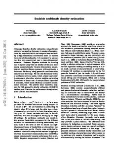
We further applied the proposed and existing methods to the problem of robot transition estimation. We used the pendulum robot and the Khepera robot simulators illustrated in Figure 2. The pendulum robot consists of wheels and a pendulum hinged to the body. The state of the pendulum robot consists of angle θ and angular velocity θ˙ of the pendulum. The amount of torque τ applied to the wheels can be controlled, by which the robot can move left or right and the state of the pendulum is changed to θ′ and θ˙′ . The task is to ˙ τ ), the transition probability density from state (θ, θ) ˙ to state (θ′ , θ˙′ ) estimate p(θ′ , θ˙′ |θ, θ, by action τ . The Khepera robot is equipped with two infra-red sensors and two wheels. The infra-red sensors dL and dR measure the distance to the left-front and right-front walls. The speed of left and right wheels vL and vR can be controlled separately, by which the robot can move forward/backward and rotate left/right. The task is to estimate p(d′L , d′R |dL , dR , vL , vR ), where d′L and d′R are the next state. The state transition of the pendulum robot is highly stochastic due to slip, friction, or measurement errors with strong heteroscedasticity. Sensory inputs of the Khepera robot suffer from occlusions and contain highly heteroscedastic noise, so the transition probability density may possess multi-modality and heteroscedasticity. Thus transition estimation of dynamic robots is a challenging task. Note that transition estimation is highly useful in model-based reinforcement learning [39]. For both robots, 100 samples were used for conditional density estimation and additional 900 samples were used for computing NLL (see Eq.(10)). The number of Gaussian components was fixed to t = 3 in MDN, and all other tuning parameters were chosen by CV based on the Kullback-Leibler (KL) error (see Section 2.5). Experimental results are summarized in Table 2, showing that LS-CDE is still useful in this challenging task of


(a) Pendulum robot.

17

(b) robot.

Khepera

Figure 2: Illustration of robots used for experiments. Table 2: Experimental results on robot transition estimation. The average and the standard deviation of NLL (see Eq.(10)) over 10 runs are described (smaller is better). The best method in terms of the mean error and comparable methods according to the twosided paired t-test at the significance level 5% are specified by bold face. Mean computation time is normalized so that LS-CDE is one. Dataset Pendulum1 Pendulum2 Khepera1 Khepera2 Time

LS-CDE 1.27 ± 0.05 1.38 ± 0.05 1.69 ± 0.01 1.86 ± 0.01 1

ϵ-KDE 2.04 ± 0.10 2.07 ± 0.10 2.07 ± 0.02 2.10 ± 0.01 0.164

MDN 1.44 ± 0.67 1.43 ± 0.58 1.90 ± 0.36 1.92 ± 0.26 1134

RKDE 11.24 ± 0.32 11.24 ± 0.32 11.03 ± 0.03 11.09 ± 0.02 0.431

robot transition estimation.

5

Conclusions and Outlook

We proposed a novel approach to conditional density estimation called LS-CDE. Our basic idea was to directly estimate the ratio of density functions without going through density estimation. LS-CDE was shown to offer a sparse solution in an analytic form and therefore is computationally efficient. A non-parametric convergence rate of the LS-CDE algorithm was also provided. Experiments on benchmark and robot-transition datasets demonstrated the usefulness of LS-CDE. The validity of the proposed LS-CDE method may be intuitively explained by the fact that it is a “one-shot” procedure (directly estimating the density ratio)—while a naive approach is two-fold (two densities are first estimated and then the ratio is estimated by plugging in the estimated densities). The plug-in approach may not be preferable since the first step is carried out without taking into account how the estimation error produced in the first step influences the second step; indeed, our experiments showed that the twostep procedure did not work properly in all cases. On the other hand, beyond these experimental results, it is important to theoretically investigate how and why the one-


18

shot approach is more suitable than the plug-in approach in conditional density estimation or in more general context of density ratio estimation. Furthermore, it is important to elucidate the asymptotic distribution of the proposed estimator, e.g., following the line of the papers [11, 27]. We used a regularizer expressed in terms of the density-ratio function in the theoretical analysis in Section 2.4, while the ℓ2 -norm of the parameter vector was adopted in the practical procedure described in Section 2.3. In order to fill the gap between theory and the practical procedure, we may use, for example, the squared norm in the function space as a regularizer. However, in our preliminary experiments, we found that the use of the function space norm as the regularizer was numerically unstable. Thus, an important future topic is to further investigate the role of regularizers in terms of consistency and also numerical stability. Smoothed analysis [35, 32, 19] would be a promising approach to addressing this issue. In the proposed LS-CDE method, a direct density-ration estimation method based on the squared-loss called unconstrained Least-Squares Importance Fitting (uLSIF) [17, 18] was applied to conditional density estimation. Similarly, applying the direct densityration estimation method based on the log-loss called the Kullback-Leibler Importance Estimation Procedure (KLIEP) [37, 38, 28, 29, 43, 44, 48], we can obtain a log-loss variant of the proposed method. A valiant of the KLIEP method explored in the papers [43, 44] uses a log-linear model (a.k.a. a maximum entropy model [16]) for density ratio estimation: rbα (x, y) := ∫

exp(α⊤ ϕ(x, y)) . exp(α⊤ ϕ(x, y ′ ))dy ′

Applying this log-linear KLIEP method to conditional density estimation is actually equivalent to maximum likelihood estimation of conditional densities for log-linear models (for structured output, it is particularly called a conditional random field [23]): [ n ] ∑ max log rbα (xi , y i ) . α∈Rb

i=1

A crucial fact regarding conditional density estimation is that the ∫ maximum-likelihood ⊤ ′ ′ normalization factor exp(α ϕ(x, y ))dy needs to be included in the model; otherwise the likelihood tends to infinity. On the other hand, the proposed method (based on the squared-loss) does not require the normalization factor to be included in the optimization problem. This is evidenced by the fact that, without the normalization factor, the proposed LS-CDE estimator is still consistent (see Section 2.4). This highly contributes to simplifying the optimization problem (see Eq.(5)); indeed, by choosing the linear density ratio model (1), the solution can be obtained analytically, as shown in Eq.(6). This is a significant advantage of the proposed method over standard maximum-likelihood conditional density estimation. An interesting theoretical research direction along this line would be to generalize the loss function to a broader class, for example, the f -divergences [1, 7]. An approach based on the paper [28] would be a promising direction to pursue.


19

When dX = 1, dY = 1, and the true ratio r is twice differentiable, the convergence rate of ϵ-KDE is ∥b r − r∥2 = Op (n−1/3 ), given that the bandwidth ϵ is optimally chosen [15]. On the other hand, Theorem 1 and the discussions before the theorem in the current paper imply that our method can achieve 1 1 − Op (n (dX +dY )/p+2 log n) = Op (n− 2/p+2 log n), where p ≥ 2. Therefore, if we choose a model such that p > 2 and the true ratio r is contained, the convergence rate of our proposed method dominates that of ϵ-KDE. This is because ϵ-KDE just takes the average around the target point x and hence it does not capture higher order smoothness of the target conditional density. On the other hand, our method can utilize the information of higher order smoothness by properly choosing the degree of smoothness with cross-validation. In the experiments, we used the common width for all Gaussian basis functions (9) in the proposed LS-CDE procedure. As shown in Section 2.4, the proposed method is consistent even with the common Gaussian width. However, in practice, it may be more flexible to use different Gaussian widths for different basis functions. Although our method in principle allows the use of different Gaussian widths, this in turn makes cross-validation computationally harder. A possible measure for this issue would be to also learn the Gaussian widths from the data together with coefficients. An expectationmaximization approach to density ratio estimation based on the log-loss for Gaussian mixture models has been explored [48], which allows us to learn the Gaussian covariances in an efficient manner. Developing a squared-loss variant of this method could produce a useful variant of the proposed LS-CDE method. As explained in Section 2.7, LS-CDE can take advantage of the semi-supervised learning setup [5], although this was not explored in the current paper. Thus it is important to investigate how the performance of LS-CDE is improved under semi-supervised learning scenarios both in theoretically and experimentally. Although we focused on conditional density estimation in this article, one may have interests in substantially simpler tasks such as error bar estimation and confidential interval estimation. Investigating whether the current line of research can be adapted to solving such simpler problems with higher accuracy is an important future issue. Even though the proposed approach was shown to work well in experiments, its performance (and also the performance of any other non-parametric approaches) is still poor in high-dimensional problems. Thus, a further challenge is to improve the accuracy in high-dimensional cases. Application of a dimensionality reduction idea in density ratio estimation [36] would be a promising direction to address this issue. Another possible future work from the application point of view would be the use of the proposed method in reinforcement learning scenarios, since a good transition model can be directly used for solving Markov decision problems in continuous and multi-dimensional domains [24, 39]. Our future work will explore this issue in more detail.


20

Acknowledgments We thank fruitful comments from anonymous reviewers. MS was supported by AOARD, SCAT, and the JST PRESTO program.

References [1] S.M. Ali and S.D. Silvey, “A general class of coefficients of divergence of one distribution from another,” Journal of the Royal Statistical Society, Series B, vol.28, no.1, pp.131–142, 1966. [2] A. Basu, I.R. Harris, N.L. Hjort, and M.C. Jones, “Robust and efficient estimation by minimising a density power divergence,” Biometrika, vol.85, no.3, pp.540–559, 1998. [3] S. Bickel, M. Br¨ uckner, and T. Scheffer, “Discriminative learning for differing training and test distributions,” Proceedings of the 24th International Conference on Machine Learning, pp.81–88, 2007. [4] C.M. Bishop, Pattern Recognition and Machine Learning, Springer, New York, NY, USA, 2006. [5] O. Chapelle, B. Schölkopf, and A. Zien, eds., Semi-Supervised Learning, MIT Press, Cambridge, 2006. [6] K.F. Cheng and C.K. Chu, “Semiparametric density estimation under a two-sample density ratio model,” Bernoulli, vol.10, no.4, pp.583–604, 2004. [7] I. Csiszár, “Information-type measures of difference of probability distributions and indirect observation,” Studia Scientiarum Mathematicarum Hungarica, vol.2, pp.229–318, 1967. [8] A.P. Dempster, N.M. Laird, and D.B. Rubin, “Maximum likelihood from incomplete data via the EM algorithm,” Journal of the Royal Statistical Society, series B, vol.39, no.1, pp.1–38, 1977. [9] D. Edmunds and H. Triebel, eds., Function Spaces, Entropy Numbers, Differential Operators, Cambridge Univ Press, 1996. [10] J. Fan, Q. Yao, and H. Tong, “Estimation of conditional densities and sensitivity measures in nonlinear dynamical systems,” Biometrika, vol.83, no.1, pp.189–206, 1996. [11] S. Geman and C.R. Hwang, “Nonparametric maximum likelihood estimation by the method of sieves,” The Annals of Statistics, vol.10, no.2, pp.401–414, 1982.


21

[12] W. Härdle, M. M¨ uller, S. Sperlich, and A. Werwatz, Nonparametric and Semiparametric Models, Springer, Berlin, 2004. [13] T. Hastie, R. Tibshirani, and J. Friedman, The Elements of Statistical Learning: Data Mining, Inference, and Prediction, Springer, New York, 2001. [14] J. Huang, A. Smola, A. Gretton, K.M. Borgwardt, and B. Schölkopf, “Correcting sample selection bias by unlabeled data,” in Advances in Neural Information Processing Systems 19, ed. B. Schölkopf, J. Platt, and T. Hoffman, pp.601–608, MIT Press, Cambridge, MA, 2007. [15] R.J. Hyndman, D.M. Bashtannyk, and G.K. Grunwald, “Estimating and visualizing conditional densities,” Journal of Computational and Graphical Statistics, vol.5, no.4, pp.315–336, 1996. [16] E.T. Jaynes, “Information theory and statistical mechanics,” Physical Review, vol.106, no.4, pp.620–630, 1957. [17] T. Kanamori, S. Hido, and M. Sugiyama, “Efficient direct density ratio estimation for non-stationarity adaptation and outlier detection,” Advances in Neural Information Processing Systems 21, ed. D. Koller, D. Schuurmans, Y. Bengio, and L. Botton, Cambridge, MA, pp.809–816, MIT Press, 2009. [18] T. Kanamori, S. Hido, and M. Sugiyama, “A least-squares approach to direct importance estimation,” Journal of Machine Learning Research, vol.10, pp.1391–1445, Jul. 2009. [19] T. Kanamori, T. Suzuki, and M. Sugiyama, “Condition number analysis of kernelbased density ratio estimation,” Tech. Rep. TR09-0006, Department of Computer Science, Tokyo Institute of Technology, Feb. 2009. [20] G.S. Kimeldorf and G. Wahba, “Some results on Tchebycheffian spline functions,” Journal of Mathematical Analysis and Applications, vol.33, no.1, pp.82–95, 1971. [21] A.N. Kolmogorov and V.M. Tikhomirov, “ε-entropy and ε-capacity of sets in function spaces,” American Mathematical Society Translations, vol.17, no.2, pp.277–364, 1961. [22] S. Kullback and R.A. Leibler, “On information and sufficiency,” Annals of Mathematical Statistics, vol.22, pp.79–86, 1951. [23] J. Lafferty, A. McCallum, and F. Pereira, “Conditional random fields: Probabilistic models for segmenting and labeling sequence data,” Proceedings of the 18th International Conference on Machine Learning, pp.282–289, 2001. [24] M.G. Lagoudakis and R. Parr, “Least-squares policy iteration,” Journal of Machine Learning Research, vol.4, pp.1107–1149, 2003.


22

[25] Y. Li, Y. Liu, and J. Zhu, “Quantile regression in reproducing kernel Hilbert spaces,” Journal of the American Statistical Association, vol.102, no.477, pp.255–268, 2007. [26] A. Luntz and V. Brailovsky, “On estimation of characters obtained in statistical procedure of recognition,” Technicheskaya Kibernetica, vol.3, 1969. in Russian. [27] W.K. Newey, “Convergence rates and asymptotic normality for series estimators,” Journal of Econometrics, vol.70, no.1, pp.147–168, 1997. [28] X. Nguyen, M. Wainwright, and M. Jordan, “Estimating divergence functionals and the likelihood ratio by penalized convex risk minimization,” in Advances in Neural Information Processing Systems 20, ed. J.C. Platt, D. Koller, Y. Singer, and S. Roweis, pp.1089–1096, MIT Press, Cambridge, MA, 2008. [29] X. Nguyen, M.J. Wainwright, and M.I. Jordan, “Nonparametric estimation of the likelihood ratio and divergence functionals,” Proceedings of IEEE International Symposium on Information Theory, Nice, France, pp.2016–2020, 2007. [30] J. Qin, “Inferences for case-control and semiparametric two-sample density ratio models,” Biometrika, vol.85, no.3, pp.619–639, 1998. [31] R Development Core Team, The R Manuals, 2008. http://www.r-project.org. [32] A. Sankar, D.A. Spielman, and S.H. Teng, “Smoothed analysis of the condition numbers and growth factors of matrices,” SIAM Journal on Matrix Analysis and Applications, vol.28, no.2, pp.446–476, 2006. [33] B. Schölkopf and A.J. Smola, Learning with Kernels, MIT Press, Cambridge, MA, 2002. [34] D.W. Scott, “Remarks on fitting and interpreting mixture models,” Computing Science and Statistics, vol.31, pp.104–109, 1999. [35] D.A. Spielman and S.H. Teng, “Smoothed analysis of algorithms: Why the simplex algorithm usually takes polynomial time,” Journal of the ACM, vol.51, no.3, pp.385– 463, 2004. [36] M. Sugiyama, M. Kawanabe, and P.L. Chui, “Dimensionality reduction for density ratio estimation in high-dimensional spaces,” Neural Networks, vol.23, no.1, pp.44– 59, 2010. [37] M. Sugiyama, S. Nakajima, H. Kashima, P. von B¨ unau, and M. Kawanabe, “Direct importance estimation with model selection and its application to covariate shift adaptation,” Advances in Neural Information Processing Systems 20, ed. J.C. Platt, D. Koller, Y. Singer, and S. Roweis, Cambridge, MA, pp.1433–1440, MIT Press, 2008.


23

[38] M. Sugiyama, T. Suzuki, S. Nakajima, H. Kashima, P. von B¨ unau, and M. Kawanabe, “Direct importance estimation for covariate shift adaptation,” Annals of the Institute of Statistical Mathematics, vol.60, no.4, pp.699–746, 2008. [39] R.S. Sutton and G.A. Barto, Reinforcement Learning: An Introduction, MIT Press, Cambridge, MA, 1998. [40] I. Takeuchi, Q.V. Le, T.D. Sears, and A.J. Smola, “Nonparametric quantile estimation,” Journal of Machine Learning Research, vol.7, pp.1231–1264, 2006. [41] I. Takeuchi, K. Nomura, and T. Kanamori, “Nonparametric conditional density estimation using piecewise-linear solution path of kernel quantile regression,” Neural Computation, vol.21, no.2, pp.533–559, 2009. [42] V. Tresp, “Mixtures of gaussian processes,” Advances in Neural Information Processing Systems 13, ed. T.K. Leen, T.G. Dietterich, and V. Tresp, pp.654–660, MIT Press, 2001. [43] Y. Tsuboi, H. Kashima, S. Hido, S. Bickel, and M. Sugiyama, “Direct density ratio estimation for large-scale covariate shift adaptation,” Proceedings of the Eighth SIAM International Conference on Data Mining (SDM2008), ed. M.J. Zaki, K. Wang, C. Apte, and H. Park, Atlanta, Georgia, USA, pp.443–454, Apr. 24–26 2008. [44] Y. Tsuboi, H. Kashima, S. Hido, S. Bickel, and M. Sugiyama, “Direct density ratio estimation for large-scale covariate shift adaptation,” Journal of Information Processing, vol.17, pp.138–155, 2009. [45] A.W. van der Vaart and J.A. Wellner, Weak Convergence and Empirical Processes with Applications to Statistics, Springer, New York, NY, USA, 1996. [46] S. Weisberg, Applied Linear Regression, John Wiley, New York, NY, USA, 1985. [47] R.C.L. Wolff, Q. Yao, and P. Hall, “Methods for estimating a conditional distribution function,” Journal of the American Statistical Association, vol.94, no.445, pp.154– 163, 1999. [48] M. Yamada and M. Sugiyama, “Direct importance estimation with Gaussian mixture models,” IEICE Transactions on Information and Systems, vol.E92-D, no.10, pp.2159–2162, 2009. [49] D.X. Zhou, “The covering number in learning theory,” Journal of Complexity archive, vol.18, no.3, pp.739–767, 2002.