Least-Squares Methods for Blind Source Separation ... - CiteSeerX

Least-Squares Methods for Blind Source Separation Based on Nonlinear PCA Petteri Pajunen and Juha Karhunen Helsinki University of Technology, Laboratory of Computer and Information Science P.O.Box 2200, FIN-02015 HUT, Espoo, FINLAND Email: Petteri.Pajunen@hut., Juha.Karhunen@hut. Fax: +358-9-451 3277

Abstract

plausible requirement that the separated sources must be statistically independent (or as independent as possible). Because direct verication of the independence condition is very dicult, some suitable higher-order statistics are in practice used for achieving separation. In neural BSS methods, higher-order statistics are incorporated into processing implicitly by using suitable nonlinearities in the learning algorithms. Dierent neural approaches to BSS and to the closely related Independent Component Analysis (ICA) [3, 4] are reviewed in [5, 2]. It has turned out that fairly simple neural algorithms [4, 6, 7, 8, 10, 9, 11, 12] are able to learn a satisfactory separating solution in many instances. In particular, we have recently shown that several nonlinear PCA (Principal Component Analysis) type neural algorithms can successfully separate a number of sources on certain conditions. Blind separation using stochastic gradient type neural learning algorithms based on nonlinear PCA approaches is discussed in detail in [10]. This work is based on our earlier extensions of standard neural principal component analysis into various forms containing some simple nonlinearities [13, 14]. The idea of extending neural PCA learning rules so that some nonlinear processing is involved was more or less independently proposed by Sanger [15], Oja [16], and Xu [17]. However, neural and adaptive algorithms proposed thus far for blind source separation are typically stochastic gradient algorithms which apply a coarse instantaneous estimate of the gradient. Such algorithms are fairly simple, but they require careful choice of the learning parameters for providing acceptable performance. If the learning parameter is too small, convergence can be intolerably slow; on the other hand the algorithm may become unstable if the learning parameter is chosen too large. In this paper, we introduce ecient recursive leastsquares (RLS) type algorithms for the blind source separation problem. These algorithms minimize in a dierent

In standard blind source separation, one tries to extract unknown source signals from their instantaneous linear mixtures by using a minimum of a priori information. We have recently shown that certain nonlinear extensions of principal component type neural algorithms can be successfully applied to this problem. In this paper, we show that a nonlinear PCA criterion can be minimized using least-squares approaches, leading to computationally ecient and fast converging algorithms. Several versions of this approach are developed and studied, some of which can be regarded as neural learning algorithms. A connection to the nonlinear PCA subspace rule is also shown. Experimental results are given, showing that the least-squares methods usually converge clearly faster than stochastic gradient algorithms in blind separation problems. Keywords: Nonlinear PCA, Blind Separation, LeastSquares, Unsupervised Learning.

1 Introduction Blind signal processing has during the last years become an important application and research domain of both unsupervised neural learning and statistical signal processing. In the basic blind source separation (BSS) problem, the goal is to separate mutually statistically independent but otherwise unknown source signals from their instantaneous linear mixtures without knowing the mixing coecients. BSS techniques have applications in a wide variety of problems for example in communications, speech processing, array processing, and medical signal processing. References and a brief description of some applications of neural BSS techniques to signal and image processing can be found in [1, 2]. Blind source separation is based on the strong but often 1

only the mixtures xj (t). Some examples of source signals are speech signals (cocktail party problem), EEG signals, and digital images. Denote by x(t) = [x1 (t); : : : ; xn (t)]T the n-dimensional data vector made up of the mixtures at discrete time (or point) t. The BSS signal model can then be written in the matrix form

way the same nonlinear PCA criterion which we have used previously as a basis of separation [10]. The proposed basic algorithms use relatively simple operations, and they can still be realized using nonlinear PCA networks. The main advantage of these algorithms is that the learning parameter is determined automatically from the input data so that it becomes roughly optimal. This usually leads to a signicantly faster convergence compared with the corresponding stochastic gradient algorithms where the learning parameter must be chosen using some ad hoc rule. Recursive least-squares methods have a long history in statistics, adaptive signal processing, and control; see [18, 19]. For example in adaptive signal processing, it is well-known that RLS methods converge much faster than the standard stochastic gradient based least-mean square (LMS) algorithm at the expense of somewhat greater computational cost [18]. Similar properties hold for the RLS algorithms presented in this paper. Our basic RLS algorithms are obtained by modifying approximate RLS algorithms proposed by Yang [20] for the standard linear PCA problem. A fundamental dierence between our and Yang's algorithms is that the latter ones do not contain any nonlinearities, and hence utilize second-order statistics only. Therefore, they cannot be directly applied to blind source separation. Apart from Yang's work, some other authors (for example [21, 22]) have applied dierent RLS approaches to the standard linear PCA problem. The contents of the rest of the paper is as follows. In the next section the necessary background on the blind source separation problem and associated neural network models is briey presented. Then the nonlinear PCA criterion is shown to be a contrast function with a suitable choice of nonlinearity. Connections between the nonlinear PCA subspace criterion and the Bussgang criterion as well as the EASI algorithm are discussed. After this, we introduce the basic recursive least-squares algorithms and some variants of them. After presentation of selected experimental results, the paper ends with conclusions and some remarks.

x(t) = As(t) + n(t):

(1)

Here s(t) = [s1 (t); : : : ; sm (t)]T is the source vector, and A is a constant full-rank n  m mixing matrix whose elements are the unknown coecients of the mixtures. The additive noise term n(t) is often omitted from (1), because it is usually impossible to separate noise from the sources without some prior knowledge on noise. The number of available dierent mixtures n must be at least as large as the number of sources m. Usually m is assumed known, and the number of sources is the same as the number of mixtures (m = n). Furthermore, each source signal si (t) is assumed to be a stationary zero-mean stochastic process. Only one of the sources is allowed to have a Gaussian distribution. In practice, it is often possible to separate the sources approximately even though they are not strictly mutually independent [24]. Essentially the same data model (1) is used in Independent Component Analysis. Assumptions on the model are described in more detail in [3, 10, 23]. It is possible to extend the basic data model (1) into various directions for example to include time delays etc. Some possibilities and references are listed in [5]. In particular, various methods for handling cases where the number of mixtures is dierent (usually greater) than that of sources are discussed in [24], and suppression of noise in [25].

2.2 Neural Network Model

In neural and adaptive BSS, an m  n separating matrix B(t) is updated so that the m-vector

y(t) = B(t)x(t) (2) becomes an estimate y(t) = bs(t) of the original independent source signals. In neural realizations, y(t) is the output vector of the network, and the matrix B(t) is the total

2 Neural Blind Source Separation 2.1 The Blind Separation Problem

weight matrix between the input and output layers. Only the waveforms of the source signals can be recovered, since the estimate s^i (t) of the i:th source signal may appear in any component yj (t) of y(t). The amplitudes and signs of the estimates yj (t) may also be arbitrary due to the inherent inderminacies of the BSS problem [26]. The estimated sources are typically scaled to have a unit variance. In several BSS algorithms, the data vectors x(t) are preprocessed by whitening them through a linear transform V so that the covariance matrix Efx(t)x(t)T g becomes the

The blind source separation problem has the following basic form. Assume that there exist m zero-mean source signals s1 (t); : : : ; sm (t) that are scalar-valued and mutually statistically independent at each time instant or index value t. The original sources si (t) are unknown, and we observe n possibly noisy but dierent linear mixtures x1 (t); : : : ; xn (t) of the sources. The constant mixing coefcients are also unknown. In blind source separation, the task is to nd the waveforms fsi (t)g of the sources, using 2

3 The Nonlinear PCA Criterion

unit matrix Im . Whitening can be done in many ways, for example using standard PCA or simple adaptive neural algorithms; see [10]. After prewhitening the separation task becomes somewhat easier, because the components of the whitened vectors x(t) are already uncorrelated which is a necessary prerequisite of independence. Also the subsequent m  m separating matrix, denoted here by WT (t), can be taken orthogonal: WT (t)W(t) = Im . The total separating matrix between input and output layers is B(t) = WT (t)V(t).

3.1 The Basic Criterion

Standard principal component analysis (PCA) is a welldened and fairly unique technique, but it utilizes secondorder statistics of the data only. There exist many neural learning algorithms for performing standard PCA [28, 29]. However, the PCA problem can be solved eciently using numerical eigenvector algorithms, so that neural gradient based algorithms are often not competitive in practical applications. If the standard PCA problem is extended so that some nonlinearities are involved, the situation changes considerably. The nonlinearities introduce at least implicitly some higher-order statistics into computations. This is often desirable for non-Gaussian data, which may contain a lot of useful information in their higher-order statistics. Furthermore, neural approaches become more competitive from the computational point of view because there usually does not exist any simple algebraic solution to the nonlinear problem. These issues are discussed in more detail in [13, 14], where several simple approaches to nonlinear PCA are introduced by generalizing optimization problems leading to standard PCA. Generally, nonlinear PCA is a non-unique concept. There exist many possible nonlinear extensions of PCA which often lead to somewhat dierent solutions. In addition to [13, 14], various neural approaches to nonlinear PCA are discussed and introduced in for example [16, 17, 30, 28, 29, 31, 32, 33]. In this paper, we concentrate on a specic form of nonlinear PCA which has been turned out to be especially useful in blind source separation. This is obtained by minimizing the nonlinear PCA subspace criterion [17, 13] J1 (W) = Efkx ? Wg(WT x)k2 g (4) with respect to the m  m weight matrix W. Here g(y) denotes the vector which is obtained by applying a nonlinear function g(t) componentwise to the vector y. In the nonlinear PCA criterion (4), g(t) is usually some odd function such as g(t) = tanh(t) or g(t) = t3 . The criterion (4) was rst proposed in a more general context by Xu in [17]. Denoting the i:th column of the matrix W by wi , the criterion (4) can be written in the form

These considerations lead to a two-layer network structure with weight matrices V and WT . Feedback connections are needed in the learning phase between the neurons in each layer. In the standard stationary case, the whitening and separating matrices converge to some constant values during learning, and the network becomes purely feedforward after learning. However, the same model can be used in the general nonstationary situation by keeping these matrices time-varying. The ensuing network structure is discussed in more detail in [10]. Roughly speaking, the currently existing neural blind separation algorithms can be divided into two main groups: the methods in the rst group try to nd the total separating matrix B(t) directly, while the methods of the second group use prewhitening. Whitening has some advantages mentioned before but also disadvantages; especially if some of the source signals are very weak or the mixture matrix is ill-conditioned, prewhitening may greatly lower the accuracy of separation. In the following, we will use the notation x(t) for both whitened and non-whitened mixture vectors, explicitly mentioning when whitening is required. A simple criterion for separating prewhitened sources having the same known sign of kurtosis is the sum of kurtoses of the outputs of the network or the separating system [27]. Our approaches are related to this criterion, because it provides simple but yet suciently ecient neural algorithms. The kurtosis of the i-th output yi (t) is dened as

4 [yi (t)] = Efyi(t)4 g ? 3[Efyi (t)2 g]2 :

(3)

J1 (W) = Efkx ?

Due to the prewhitening, Efyi (t)2 g = 1, and it suces to consider the sum of the fourth moments of the outputs. This criterion is minimized for sub-Gaussian sources (for which the kurtosis is negative), and maximized for superGaussian sources (having a positive kurtosis value). For Gaussian sources, the kurtosis is zero. The theory of separation is presented in more detail in [5, 10, 27].

m X i=1

g(wiT x)wi k2 g:

(5)

This shows that the sum which tries to approximate the data vector x is linear with respect to the weight vectors wi , the nonlinearity g(t) appearing only in the coecients g(wiT x) of the expansion. This simple form of nonlinear PCA is not the best possible if the goal is to approximate the data vector x for example in data compression or 3

representation, but the coecients introduce higher-order statistics which are needed in blind separation. The criterion (4) can be approximately minimized using the stochastic gradient descent algorithm
W = [x ? Wg(WT x)]g(xT W)

30

10

9

8 10 7

0

6

5 −10 4

3

(6)

−20 2

−30 −5

This nonlinear PCA subspace rule has been independently derived in [17] and [13]. In (6),  is a positive learning parameter, and we have omitted the time index t from all the quantities for simplicity. The algorithm (6) was rst proposed by Oja et al. in [16] on heuristic grounds. For more details and related algorithms, see [16, 17, 13, 14].

−4

−3

−2

−1

0

1

2

3

4

5

1 −5

−4

−3

−2

−1

0

1

2

3

4

5

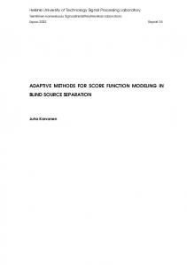
Figure 1: Left: The odd quadratic function g. Right: The derivative of g. specic nonlinearity. The orthogonality of the separating matrix W (WT W = WWT = I, where I is the unit matrix) allows us to analyze the criterion (4) in more detail for prewhitened data vectors x. In this case, one can express the criterion (4) in the form

3.2 Application to Blind Source Separation

J1 (W) = Efkx ? Wg(WT x)k2 g

In applying the criterion (4) and the algorithm (6) to the blind separation problem, it is essential that the data vectors x(t) are rst preprocessed by whitening them. Thus the nonlinear PCA learning rule is applied to BSS problems in the form
W = [x ? Wg(y)]g(yT )

11

20

= EfkWT x ? WT Wg(WT x)k2 g = Efky ? g(y)k2 g m X = Ef[yi ? g(yi )]2 g: i=1

(7)

(8)

If we now dene an odd quadratic function illustrated in Figure 1 as

where y = WT x. Later on we have justied in several papers summarized in [10] that for the prewhitened mixture vectors x(t), WT (t) becomes an orthogonal m  m separating matrix provided that all the source signals are of the same type, namely either sub-Gaussian or super-Gaussian. In practice, this condition can be mildened somewhat so that one of the sources can be of dierent type if its kurtosis has the smallest absolute value [23, 10]. In order to achieve separation, it suces that the nonlinearity g(t) is of right type [36, 10]. More precisely, for sub-Gaussian sources g(t) should grow less than linearly. Later, it is seen that this condition is closely connected with a general nonlinearity determined by the source signal density functions. We have used in our earlier experiments the sigmoidal nonlinearity g(t) = tanh(t) with good results. The robustness of the blind separation problem against choosing a non-optimal nonlinearity is discussed in [36, 26]. The nonlinear PCA rule (7) can be applied also for super-Gaussian sources using Fahlman type activation functions [38]. Alternatively, one could use the cubic nonlinearity g(t) = t3 . However, this kind of fast growing nonlinearity often requires extra measures (some kind of normalization) for keeping the algorithm stable. The separation properties of the algorithm (7) have been analyzed rigorously in simple cases in [37]. Recently it has been shown [38] that the criterion function (4) is approximately related to a separating contrast function derived in [3]. Below, we show an exact correspondence using a

(

2 g(y) = y +2 y; y  0; ?y + y; y < 0;

(9)

the criterion (8) becomes m X 2 2 J1 (W) = Ef[yi ? yi  yi ] g = Efyi4 g i=1 i=1 m X

P

(10)

The statistic J1 (W) = i Efyi4g has been rigorously shown to be a contrast in [27] under the following assumptions: all the sources have the same known sign of kurtosis, and the data have been prewhitened. Therefore, each of the global minima (there are several) of J1 correspond exactly to the separating solutions. Experimentally it has been found that local optimization of J1 usually provides the separated sources. The simple form (8) makes it easier to understand the eect of any nonlinearity to separation, and allows a comparison to known contrast functions [3]. Consider for example the sigmoidal nonlinearity g(t) = tanh(t) which has been used widely in neural separation algorithms. Inserting the Taylor series expansion tanh(t) = t ? t3 =3 + 2t5=15 ? : : : into (8) one can easily see that in this case the criterion J1 (W) actually depends on sixth order (and higher) statistics. 4

3.3 Relationships to Other Approaches

In [40] we have derived a closely related algorithm from the nonlinear PCA rule (7) as follows. For the total sepa3.3.1 Blind Equalization Using Bussgang Ap- rating matrix B = WT V, the update rule is in general proaches
B = k [
WT V + WT
V]:

The form Efky ? g(y)k2 g is similar to the Bussgang blind equalization cost [18, 39], in which the nonlinearity is chosen to be 2 0 (11) g(x) = ?Efjpxj(xg)px(x) ; x where px is the probability density function of x. Since the mixtures are whitened, the expectation Efjxj2 g = 1, and for px (x) =1= cosh(x) we get

(14)

Using the nonlinear PCA learning rule for
W and the simple whitening algorithm
V = [I ? xxT ]V

(15)

and constraining W to be orthogonal, the following algorithm is obtained for the total separating matrix B:
B = k [I ? yyT + g(y)yT ? g(y)g(yT )]B

x) = tanh(x): g(x) = sinh(x) cosh( cosh2 (x)

(16)

(12) A comparison with the EASI algorithm (13) shows that the derived algorithm (16) diers only slightly from it (the This means that (4) with g(x) = tanh(x) is a Bussgang sign of the nonlinear part g(y)yT ? g(y)g(yT ) is not imblind equalization cost for sources with a density propor- portant). In [23], the EASI algorithm is derived by making tional to px (x) = 1= cosh(x). This corresponds to a signal rather heavy but sensible approximations. with a positive kurtosis. However, in the nonlinear PCA learning rule the nonlinearity g(x) = tanh(x) makes it possible to separate signals with negative kurtosis. Con- 4 Least-Squares Algorithms for the versely, nonlinearities corresponding to signals with negNonlinear PCA Criterion ative kurtosis according to (11) can be used to separate signals with positive kurtosis using nonlinear PCA learn- 4.1 Symmetric Recursive Algorithm ing rule. The reasons for this are discussed in [40]. Although in the Bussgang blind equalization cost it is as- Our basic recursive least-squares algorithms are closely resumed that the density px is known, it has been shown lated to Yang's recent work [20], in which he has derived a that it is not necessary to exactly match the nonlinearity RLS algorithm called PAST for adaptive tracking of signal subspaces. A signal subspace models the "signal" part in with the source density [36]. the data, and it is essentially the same as a PCA subspace Based on Lambert's work [39], we have also shown in of suitable dimension. Signal subspaces are used especially 2 [40] that the minimization of the cost Efky ? g(y)k g can be interpreted as nding an extremal point of the sum of in linear eigenvector methods of array processing and sinusoidal frequency estimation. negentropies Yang derives his PAST algorithm from the cost function X J = E flog py (yi )= log pG (yi )g J (W) = Efkx ? WWT xk2 g: (17) i

2

i

This criterion diers from the nonlinear PCA criterion (4) in that the nonlinear function g(t) is lacking from it. Therefore, the criterion (17) does not take into account any higher-order statistics in the data even implicitly. The cost function (17) has been considered in several earlier papers dealing with PCA neural networks [34, 13, 14, 28, 17, 35]. It is well-known that the minimum of (17) is provided by any orthogonal matrix W whose columns span the PCA subspace dened by the principal eigenvectors of the data covariance matrix EfxxT g (for zero mean data). Some of these results have been rederived in [41] together with a convergence analysis of the PAST algorithms. In this paper we extend Yang's PAST algorithm so that it can be used for minimizing the nonlinear cost function (4), and apply the resulting modied algorithm to

Here py is the probability density function of the i:th output signal yi and pG is the density of the Gaussian distribution with the same variance as yi . Thus minimization of the nonlinear PCA criterion for prewhitened data is also closely related to a meaningful information-theoretic criterion, since the sum of negentropies measures the nonGaussianity of the outputs. i

3.3.2 The EASI Algorithm

A well-known stochastic gradient algorithm for blind separation without prewhitening is the EASI algorithm introduced by Cardoso and Laheld in [23]. The general update formula for the separating matrix B is in EASI
B = k [I ? yyT ? g(y)yT + yg(yT )]B:

(13) 5

blind source separation. Our modied symmetric (or sub- 4.2 Sequential Recursive Algorithm space type) nonlinear PAST algorithm adapted for the The algorithm (18) updates the whole weight matrix BSS problem reads as follows: W(t) simultaneously, treating all the weight vectors or the columns w1 (t); : : : ; wm (t) of the matrix W(t) in a T z(t) = g(W (t ? 1)x(t)) = g(y(t)); symmetric way. Alternatively, we can compute the weight h(t) = P(t ? 1)z(t); vectors wi(t) in a sequential manner using a deation techm(t) = h(t)=( + zT (t)h(t)); nique. The resulting algorithm has the following form: P(t) = 1 Tri P(t ? 1) ? m(t)hT (t) ; x1 (t) = x(t); For each i = 1; : : : ; m compute e(t) = x(t) ? W(t ? 1)z(t); zi (t) = g(wiT (t ? 1)xi (t)); W(t) = W(t ? 1) + e(t)mT (t): (18) di (t) = di (t ? 1) + [zi (t)]2 ; The constant 0 <  1 is a forgetting term which should ei (t) = xi (t) ? wi(t ? 1)zi(t); be close to unity. The notation Tri means that only the wi (t) = wi(t ? 1) + ei (t)[zi (t)=di (t)]; upper triangular part of the argument is computed and its xi+1 (t) = xi (t) ? wi(t)zi (t): (20) transpose is copied to the lower triangular part, making thus the matrix P(t) symmetric. The simplest way to choose the initial values is to set both W(0) and P(0) to Here again the data vectors x(t) must be prewhitened, and m  m unit matrices. According to the theory, the data di (t) provides an individual learning parameter 1=di (t) for vectors x(t) must be prewhitened prior to using them in each weight vector wi (t) from a simple recursion formula. Let us now compare the algorithms (18) and (20) to the the algorithm (18). The symmetric algorithm (18) can be regarded either nonlinear PCA subspace learning rule (7). Consider for as a neural network learning algorithm or adaptive signal ease of comparison the single neuron case m = 1. Both processing algorithm. It does not require any matrix inver- the symmetric and sequential versions then reduce to the sions, because the most complicated operation is division algorithm by a scalar. Especially the sequential version discussed in the next subsection becomes relatively simple when writw(t) = w(t ? 1) + d(1t) [x(t) ? w(t ? 1)z(t)]z(t) (21) ten out for each weight vector. The algorithm (18) and its modied versions can be deT rived using the following principles [20, 19]. Because the where z (t) = g(w (t ? 1)x(t)) = g(y(t)), and expectation in (4) is unknown, it is rst replaced by the d(t) = d(t ? 1) + [z (t)]2 : (22) sum over the last samples, leading to the respective leastsquares criterion. Then we approximate the unknown vec- The algorithm (21) is exactly the same as the nonlinear tor g(WT (t)x(t)) by the vector z(t) = g(WT (t ? 1)x(t)). PCA learning rule (7) except for the scalar learning paThis vector can be easily computed because the estimated rameter. In (21), the learning parameter 1=d(t) is deterweight matrix WT (t ? 1) from the previous iteration step mined automatically from the properties of the data using t ? 1 is already known. The approximation error is usually the recursion (22) so that it becomes roughly optimal due rather small after initial convergence, because the update to the minimization of the least-squares criterion (19). On term
W(t) then becomes small compared to weight ma- the other hand, in (7) the learning parameter (t) is usutrix W(t). These considerations yield the modied least- ally a constant which is chosen by a somewhat ad hoc squares type criterion manner or by tuning it to the average properties of the data. It is just this nearly optimal choice of the learnt X t ? i 2 ing parameter that yields the algorithms (18) and (20) J3 (W(t)) = kx(i) ? W(t)z(i)k : (19) their superior convergence properties compared to stani=1 dard stochastic gradient type learning algorithms such as If the forgetting factor = 1, all the samples are given (7). the same weight, and no forgetting of old data takes place. The original PAST algorithms [20] which estimate either Choosing < 1 is useful especially in tracking nonstation- the PCA subspace or the PCA eigenvectors themselves ary changes in the sources. The cost function (19) is now have a similar relationship to the well-known Oja's oneof the standard form used in recursive least-squares meth- unit rule [28, 42], which is the seminal neural algorithm for ods. Any of the available algorithms [19] can be used for learning the rst PCA eigenvector. However, they cannot solving the weight matrix W(t) iteratively. We have in be applied to the BSS problem because no higher-order this paper used the ecient algorithm (18). statistics or nonlinearities are used. 6

4.3 Batch Versions

4.3.2 Sequential Batch Algorithm It is possible to nd the weight matrix W one column at

4.3.1 Symmetric Batch Algorithm

a time by minimizing the cost function

The previous considerations and the form of the cost function (4) suggest straightforward batch algorithms for optimizing the matrix W. These algorithms are no longer neural because they are non-adaptive and use all the data vectors during each iteration cycle. However, they are derived by iteratively minimizing the same nonlinear PCA criterion as before. If it is assumed for the moment that the matrix W in the term g(WT x) is a constant, (4) can be regarded as the least-squares error for the linear model

X = Wg(WT X) + e = WG + e;

Js = E[kx ? wg(wT x)k2 ];

(28)

where w is a weight vector. A minimizing solution w^ gives one of the separated sources as the inner product w^ T x. We can directly use the derivation of the symmetric algorithm by replacing the matrix W by the weight vector w. The linear updating step (27) becomes P w = Pg(gy((yj())j ))x(2j ) :

(23)

(29)

Once w is found, the algorithm is repeated with a different initial value for w until all the sources have been where e is the modeling error or noise term, the matrix found. After each iteration, w must be orthogonalized against the previously found weight vectors using for exG = [g(WT x(1)); : : : ; g(WT x(N ))] (24) ample the well-known Gram-Schmidt procedure [28, 43]. This ensures that the algorithm does not converge to a is a constant, and the data matrix X is dened by previously found vector (see [44]). It seems that in practice it is better to compute only the numerator in (29), X = [x(1); : : : ; x(N )]: (25) and then normalize w explicitly by w = w=kwk. Now a new value for the weight matrix W can be computed by minimizing the least-squares error kek2 for the 5 Experimental Results linearized model (23). This is equivalent to nding the best approximate solution to the linear matrix equation In the experiments below, we used four sub-Gaussian source signals: a ramp, a sinusoid, a binary signal, and X = WG (26) uniformly distributed white noise. Actually three of the sources are deterministic for easy visual comparison and in the least-squares error sense. It is well-know (see for ex- inspection of the results. These sources were mixed linample [43], p. 54) that the optimal solution to this problem early using a 4  4 mixing matrix, whose elements were ^ = XG+ , where G+ is the pseudoinverse of G. Now Gaussian random numbers. is W G actually depends on W, but we can anyway determine In the rst experiment the convergence speed of dif^ using the following iterative symmetric algorithm: ferent algorithms was compared. The nonlinear PCA subW space rule was compared with the proposed recursive least1. Choose an initial value for W. squares algorithms. Convergence was measured by the following cost C , which is similar to the one proposed in [6]: 2. Compute G using the current value of W. X X jpij j2 ? 1) ( (30) D = 3. Update the weight matrix W: max jp j2

W = XGT (GGT )?1 = XG+

j

i

(27)

+

X X

j

p

(

C= D

4. Continue iteration from step 2 until convergence

k ik jpij j2

2 i maxk jpkj j

? 1)

The elements pij are from the total system matrix P = WT VA, where V is the whitening matrix. For a separat-

The basic idea is to treat the weight matrix in the argument of g as a constant, and then optimize with respect to the weight matrix W outside g using the standard linear least-squares method. After sucient number of iterations, W should converge close to a local minimum of (4). Recall that these local minima yield a separating matrix W for prewhitened mixture vectors v.

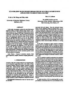
ing solution, the value of C is zero and positive otherwise. A typical learning rate  = 0:01 was chosen and for the RLS algorithms, a forgetting factor = 1 ?  = 0:99 was chosen. All algorithms used the same data, 1000 samples of four linear mixtures of four sub-Gaussian sources.

7

3

2.5

3

2 2.5 GENERALIZED PERMUTATION INDEX

1.5

1

0.5

0

0

100

200

300

400

500

600

700

800

900

2

1.5

1

1000 0.5

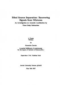
Figure 2: The convergence speed of the recursive leastsquares algorithms is compared with the nonlinear PCA subspace rule using  = 0:01 and = 0:99. Solid: Nonlinear PCA subspace rule. Dashed: Symmetric RLS al- Figure 3: The convergence of the recursive least-squares gorithm. Dotted: Sequential RLS algorithm. The curves algorithms is compared with the nonlinear PCA subspace show the performace index (30) as a function of iterations. rule using  = 0:02 and = 0:98. Solid: Nonlinear PCA subspace rule. Dashed: Symmetric RLS algorithm. DotSequential RLS algorithm. The curves show the perIn gure 2, the value of the performance index C is de- ted: formace index (30) as a function of iterations. picted as a function of iterations. The convergence curves clearly show that the recursive least-squares algorithms perform better than the nonlinear PCA subspace rule. Furthermore, the symmetric algorithm converges faster than the sequential version. In a similar experiment with the parameter values  = 0:02 and = 0:98 the results were similar (see Figure 3). In another experiment, the sequential batch algorithm (29) using explicit normalization was compared to the nonlinear PCA learning rule (7) by nding one basis vector w of four mixtures of four sub-Gaussian sources. The number of data vectors x(i) was 100, and each algorithm was run 50 cycles. In (7) one cycle means using each sample once (100 iterations). We used the sigmoidal nonlinearity g(y) = tanh(y). Figure 4 shows that the proposed batch algorithm converges faster and achieves a better nal accuracy. The experimental results presented above are typical ones achieved using these algorithms. In all the computer simulations that we have made thus far the proposed leastsquares algorithms (18) and (20) converged faster than the existing adaptive neural BSS algorithms. The dierence in the convergence speed is often of the order of magnitude or even higher compared with the nonlinear PCA subspace Figure 4: Solid line: Sequential batch algorithm. Dashed rule (and other stochastic gradient type algorithms that line: Nonlinear PCA algorithm. The x-axis represents the number of oating point operations and the y-axis signalhave a roughly similar performance [5]). ratio of the separated source vs. the correspondIn general, the nal accuracy achieved by RLS algo- to-noise ing original source. rithms can be improved in stationary situations by increasing the forgetting parameter from its initial value (say = 0:95) closer to unity after initial convergence has been taken place. Similarly, in gradient type algorithms 0

0

100

200

300

400

500 600 ITERATIONS

700

800

900

1000

44 42 40 38

SNR (dB)

36 34 32 30 28 26

24 0

8

2

4

6

8

10 FLOPS

12

14

16

18 4

x 10

the value of the learning parameter  can be decreased with time for achieving a better accuracy. The convergence speed of the nonlinear PCA subspace rule (6) may depend greatly on the chosen initial values of the weight vectors [38]. The least-squares algorithms introduced in this paper are more robust in this respect. Although the proposed adaptive RLS algorithms utilize a xed nonlinearity g, it is straightforward to extend the algorithms so that the nonlinearity is not xed. This can be done e.g. by estimating the sign of the kurtosis of the outputs online (see [45, 46]), which makes it possible to separate sources with dierent sign of kurtosis. All the adaptive learning algorithms can be used also for simultaneous tracking and separation of sources in nonstationary situations. This problem is very dicult but important in practice. We have presented some tracking experiments with the proposed RLS type algorithms in [47, 48].

Int. Conf. on Acoustics, Speech, and Signal Processing (ICASSP'97), Munich, Germany, April 1997, pp. 131-134.

[2] E. Oja, J. Karhunen, A. Hyvärinen, R. Vigário, and J. Hurri, Neural independent component analysis approaches and applications, in Brain-like Computing and Intelligent Information Systems, S.-I. Amari and N. Kasabov (Eds.), Springer-Verlag, Singapore, 1998, pp. 167-188. [3] P. Comon, Independent component analysis - a new concept?, Signal Processing, vol. 36, pp. 287-314, 1994. [4] C. Jutten and J. Herault, Blind separation of sources, part I: an adaptive algorithm based on neuromimetic architecture, Signal Processing, vol. 24, no. 1, pp. 1-10, July 1991. [5] J. Karhunen, Neural approaches to independent component analysis and source separation, in Proc. 4th European Symp. on Articial Neural Networks (ESANN'96), Bruges, Belgium, April 1996, pp. 249266.

6 Conclusions

In this paper we have introduced several new algorithms for blind source separation and possible other applications based on a nonlinear PCA criterion. In particular, we have discussed minimization of the nonlinear PCA cost function [6] (4) using approximative least-squares approaches. The proposed nonlinear recursive least-squares type algorithms (18) and (20) provide faster convergence in blind source separation compared with the corresponding stochastic gradient algorithms, in the same sense as recursive leastsquares (RLS) algorithms are fast compared with stochas- [7] tic gradient LMS algorithms in adaptive ltering [18]. According to the experiments made thus far, they provide a very good performance with a fairly low computational load. In some instances, it may be computationally more [8] ecient to use the batch versions of the least-squares algorithms. We have also mentioned connections of the nonlinear PCA criterion to some well-known existing approaches such as Bussgang methods in blind equalization and the adaptive EASI blind source separation algorithm. [9] Together with earlier works, the results in this paper demonstrate that nonlinear PCA is a versatile and useful starting point for blind signal processing with close connections to some other well-known approaches. There exist several possibilities for further research such as taking into account robustness, time delays etc. [10]

References

S. Amari, A. Cichocki, and H. Yang, A new learning algorithm for blind signal separation, in Advances in Neural Information Processing Systems 8, D.S. Touretzky et al. (Eds.). Cambridge, MA: MIT Press, 1996, pp. 757-763. A. Bell and T. Sejnowski, An informationmaximisation approach to blind separation and blind deconvolution, Neural Computation, vol. 7, pp. 11291159, 1995. A. Cichocki and R. Unbehauen, Robust neural networks with on-line learning for blind identication and blind separation of sources, IEEE Trans. on Circuits and Systems-1, vol. 43, pp. 894-906, November 1996. L. Wang, J. Karhunen, and E. Oja, A bigradient optimization approach for robust PCA, MCA, and source separation, in Proc. 1995 IEEE Int. Conf. on Neural Networks, Perth, Australia, November 1995, pp. 1684-1689. J. Karhunen, E. Oja, L. Wang, R. Vigario, and J. Joutsensalo, A class of neural networks for independent component analysis, IEEE Trans. on Neural Networks, vol. 8, pp. 486-504, May 1997.

[1] J. Karhunen, A. Hyvärinen, R. Vigário, J. Hurri, and [11] G. Deco and D. Obradovic, An Information-Theoretic E. Oja, Applications of neural blind separation to Approach to Neural Computing. New York: Springersignal and image processing, in Proc. 1997 IEEE Verlag, 1996. 9

[12] M. Girolami and C. Fyfe, A temporal model of linear anti-hebbian learning, Neural Processing Letters, vol. 4, pp. 139-148, 1996. [13] J. Karhunen and J. Joutsensalo, Representation and separation of signals using nonlinear PCA type learning, Neural Networks, vol. 7, no. 1, pp. 113-127, 1994. [14] J. Karhunen and J. Joutsensalo, Generalizations of principal component analysis, optimization problems, and neural networks, Neural Networks, vol. 8, no. 4, pp. 549-562, 1995. [15] T. Sanger, An optimality principle for unsupervised learning, in D. Touretzky (Ed.), Advances in Neural Information Processing Systems 1, Morgan Kaufmann, Palo Alto, CA, 1989, pp. 11-19. [16] E. Oja, H. Ogawa, and J. Wangviwattana, Learning in nonlinear constrained Hebbian networks. In T. Kohonen et al. (Eds.), Articial Neural Networks (Proc. ICANN'91, Espoo, Finland), North-Holland, Amsterdam, 1991, pp. 385-390. [17] L. Xu, Least mean square error reconstruction principle for self-organizing neural-nets, Neural Networks, vol. 6, pp. 627-648, 1993. [18] S. Haykin, Adaptive Filter Theory, 3rd ed. PrenticeHall, 1996. [19] J. Mendel, Lessons in Estimation Theory for Signal Processing, Communications, and Control. Englewood Clis: Prentice-Hall, 1995. [20] B. Yang, Projection approximation subspace tracking, IEEE Trans. on Signal Processing, vol. 43, pp. 95-107, January 1995. [21] S. Bannour and M. Azimi-Sadjadi, Principal component extraction using recursive least squares learning, IEEE Trans. on Neural Networks, vol. 6, pp. 457-469, March 1995. [22] W. Kasprzak and A. Cichocki, Recurrent least squares learning for quasi-parallel principal component analysis, in Proc. 4th European Symp. on Articial Neural Networks (ESANN'96), Bruges, Belgium, April 1996, pp. 223-228. [23] J.-F. Cardoso and B. Laheld, Equivariant adaptive source separation, IEEE Trans. on Signal Processing, vol. 44, pp. 3017-3030, December 1996. [24] A. Cichocki, J. Karhunen, W. Kasprzak, and R. Vigario, On neural blind separation with unequal numbers of sources, sensors, and outputs, manuscript submitted to a journal, November 1996.

[25] J. Karhunen, A. Cichocki, W. Kasprzak, and P. Pajunen, On neural blind separation with noise suppression and redundancy reduction, Int. J. of Neural Systems, vol. 8, no. 2, pp. 219-237, 1997. [26] J.-F. Cardoso, Entropic contrasts for source separation, to appear as Chapter 2 in S. Haykin (Ed.), Adaptive Unsupervised Learning., 1998. [27] E. Moreau and O. Macchi, High-order contrasts for self-adaptive source separation, Int. J. of Adaptive Control and Signal Processing, vol. 10, pp. 19-46, 1996. [28] K. Diamantaras and S. Kung, Principal Component Networks - Theory and Applications. New York: John Wiley, 1996. [29] F.-L. Luo and R. Unbehauen, Applied Neural Networks for Signal Processing. Cambridge: Cambridge Univ. Press, 1997. [30] L. Xu, Theories for unsupervised learning: PCA and its nonlinear extensions, in Proc. IEEE Int. Conf. on Neural Networks (ICNN'94), Orlando, Florida, JuneJuly 1994, pp. 1252a-1257. [31] F. Palmieri, Hebbian learning and self-association in nonlinear neural networks, in Proc. IEEE Int. Conf. on Neural Networks (ICNN'94), Orlando, Florida, June-July 1994, pp. 1258-1263. [32] A. Sudjianto, M. Hassoun, and G. Wasserman, Extensions of principal component analysis for nonlinear feature extraction, in Proc. 1996 IEEE Int. Conf. on Neural Networks (ICNN'96), Washington D.C., USA, June 1996, pp. 1433-1438. [33] R. Hecht-Nielsen, Data manifolds, natural coordinates, replicator neural networks, and optimal source coding, in Proc. 1996 Int. Conf. on Neural Information Processing (ICONIP'96), Hong Kong, September 1996, pp. 1207-1210. [34] P. Baldi and K. Hornik, Neural networks and principal component analysis: learning from examples without local minima, Neural Networks, vol. 2, pp. 53-58, 1989. [35] F. Palmieri and J. Zhu, Self-association and Hebbian learning in linear neural networks, IEEE Trans. on Neural Networks, vol. 6, pp. 1165-1184, September 1995. [36] J.-F. Cardoso, Infomax and maximum likelihood for blind source separation, IEEE Signal Processing Letters, vol. 4, pp. 112-114, April 1997.

10

[37] E. Oja, The Nonlinear PCA learning rule in independent component analysis, Neurocomputing, vol. 17, no. 1, pp. 25-46, 1997. [38] M. Girolami and C. Fyfe, Stochastic ICA contrast maximisation using Oja's nonlinear PCA algorithm, submitted to Int. J. Neural Systems, July 1996. [39] R. Lambert, Multichannel Blind Deconvolution: FIR Matrix Algebra and Separation of Multipath Mixtures. Ph.D. dissertation, Univ. of Southern California, Dept. of Electrical Eng., May 1996. [40] J. Karhunen, P. Pajunen, and E. Oja, The nonlinear PCA criterion in blind source separation: relations with other approaches, to appear in Neurocomputing, 1998. [41] B. Yang, Asymptotic convergence analysis of the projection approximation subspace tracking algorithms, Signal Processing, vol. 50, pp. 123-146, 1996. [42] E. Oja, A simplied neuron model as a principal component analyzer, J. of Mathematical Biology, vol. 15, pp. 267-273, 1982. [43] T. Kohonen, Self-Organization and Associative Memory, 3rd ed. Springer-Verlag, New York, 1989. [44] A. Hyvärinen and E. Oja, A fast xed-point algorithm for independent component analysis, Neural Computation, vol. 9, no. 7, pp. 1483-1492, 1997. [45] J. Karhunen and P. Pajunen, Hierarchic nonlinear PCA algorithms for neural blind source separation, in NORSIG 96 Proceedings - 1996 IEEE Nordic Signal Processing Symposium, pp. 71-74, 1996. [46] A. Hyvärinen and E. Oja, Independent component analysis by general nonlinear Hebbian-like learning rules, in Signal Processing, vol. 64, no. 3, pp. 301313, 1998. [47] J. Karhunen and P. Pajunen, Blind source separation using least-squares type adaptive algorithms, in Proc. 1997 IEEE Int. Conf. on Acoustics, Speech, and Signal Processing (ICASSP'97), Munich, Germany, April 1997, pp. 3361-3364. [48] J. Karhunen and P. Pajunen, Blind source separation and tracking using nonlinear PCA criterion: a leastsquares approach, in Proc. 1997 Int. Conf. on Neural Networks (ICNN'97), Houston, Texas, June 1997, pp. 2147-2152.

11