For example, the set of admissible controls could be the set of piecewise ..... In
MATLAB K and P can be computed using. [K,P] = lqr(A,B,Q,R); ... Suppose the
state feedback cost function is. J = ∫. ∞. 0 hu2 ..... equation (DARE). A. T. PA − P
− A.
ELEC4410
Control Systems Design Lecture 22: Introduction to Optimal Control and Estimation Julio H. Braslavsky
[email protected]
School of Electrical Engineering and Computer Science The University of Newcastle
The University of Newcastle
Lecture 22: Introduction to Optimal Control and Estimation – p. 1
Outline Introduction The basic optimal control problem Optimal linear quadratic state feedback Optimal linear quadratic state estimation
The University of Newcastle
Lecture 22: Introduction to Optimal Control and Estimation – p. 2
Introduction The state feedback and observer design approach is a fundamental tool in the control of state equation systems. However, it is not always the most useful method. Three obvious difficulties are: The translation from design specifications (maximum desired over and undershoot, settling time, etc.) to desired poles is not always direct, particularly for complex systems; what is the best pole configuration for the given specifications?
The University of Newcastle
Lecture 22: Introduction to Optimal Control and Estimation – p. 3
Introduction The state feedback and observer design approach is a fundamental tool in the control of state equation systems. However, it is not always the most useful method. Three obvious difficulties are: The translation from design specifications (maximum desired over and undershoot, settling time, etc.) to desired poles is not always direct, particularly for complex systems; what is the best pole configuration for the given specifications? In MIMO systems the state feedback gains that achieve a given pole configuration is not unique. What is the best K for a given pole configuration?
The University of Newcastle
Lecture 22: Introduction to Optimal Control and Estimation – p. 3
Introduction The state feedback and observer design approach is a fundamental tool in the control of state equation systems. However, it is not always the most useful method. Three obvious difficulties are: The translation from design specifications (maximum desired over and undershoot, settling time, etc.) to desired poles is not always direct, particularly for complex systems; what is the best pole configuration for the given specifications? In MIMO systems the state feedback gains that achieve a given pole configuration is not unique. What is the best K for a given pole configuration? The eigenvalues of the observer should be chosen faster than those of the closed-loop system. Is there any other criterion available to help decide one configuration over another?
The University of Newcastle
Lecture 22: Introduction to Optimal Control and Estimation – p. 3
Introduction The state feedback and observer design approach is a fundamental tool in the control of state equation systems. However, it is not always the most useful method. Three obvious difficulties are: The translation from design specifications (maximum desired over and undershoot, settling time, etc.) to desired poles is not always direct, particularly for complex systems; what is the best pole configuration for the given specifications? In MIMO systems the state feedback gains that achieve a given pole configuration is not unique. What is the best K for a given pole configuration? The eigenvalues of the observer should be chosen faster than those of the closed-loop system. Is there any other criterion available to help decide one configuration over another? The methods that we will now introduce give answers to these questions. We will see how the state feedback and observer gains can be found in an optimal way. The University of Newcastle
Lecture 22: Introduction to Optimal Control and Estimation – p. 3
Some References for Further Reading References [1] G.C. Goodwin, S.F. Graebe, and M.E. Salgado. Control System Design. Prentice Hall, 2001. [2] J.S. Bay. Fundamentals of Linear State Space Systems. McGraw-Hill, 1999. [3] J.M. Maciejowski. Multivariable Feedback Design. Addison-Wesley Publishing Company, 1991. [4] B.D.O. Anderson and J.B. Moore. Optimal Control. Linear quadratic methods. Prentice-Hall International, 1989. [5] Kemin Zhou, John C. Doyle, and Keith Glover. Robust and optimal control. Prentice Hall, 1996.
The University of Newcastle
Lecture 22: Introduction to Optimal Control and Estimation – p. 4
The Basic Optimal Control Problem What does optimal mean? Optimal means doing a job in the best possible way. However, before starting a search for an optimal solution, the job must be defined
The University of Newcastle
Lecture 22: Introduction to Optimal Control and Estimation – p. 5
The Basic Optimal Control Problem What does optimal mean? Optimal means doing a job in the best possible way. However, before starting a search for an optimal solution, the job must be defined a mathematical scale must be established to quantify what we mean by best
The University of Newcastle
Lecture 22: Introduction to Optimal Control and Estimation – p. 5
The Basic Optimal Control Problem What does optimal mean? Optimal means doing a job in the best possible way. However, before starting a search for an optimal solution, the job must be defined a mathematical scale must be established to quantify what we mean by best the possible alternatives must be spelled out. Unless these qualifiers are clear and consistent, a claim that a system is optimal is really meaningless.
The University of Newcastle
Lecture 22: Introduction to Optimal Control and Estimation – p. 5
The Basic Optimal Control Problem What does optimal mean? Optimal means doing a job in the best possible way. However, before starting a search for an optimal solution, the job must be defined a mathematical scale must be established to quantify what we mean by best the possible alternatives must be spelled out. Unless these qualifiers are clear and consistent, a claim that a system is optimal is really meaningless. A crude, inaccurate system might be considered optimal because it is inexpensive, is easy to fabricate, and gives adequate performance.
The University of Newcastle
Lecture 22: Introduction to Optimal Control and Estimation – p. 5
The Basic Optimal Control Problem What does optimal mean? Optimal means doing a job in the best possible way. However, before starting a search for an optimal solution, the job must be defined a mathematical scale must be established to quantify what we mean by best the possible alternatives must be spelled out. Unless these qualifiers are clear and consistent, a claim that a system is optimal is really meaningless. A crude, inaccurate system might be considered optimal because it is inexpensive, is easy to fabricate, and gives adequate performance. Conversely, a very precise and elegant system could be rejected as nonoptimal because it is too expensive or it is too heavy or would take too long to develop. The University of Newcastle
Lecture 22: Introduction to Optimal Control and Estimation – p. 5
The Basic Optimal Control Problem The mathematical statement of the optimal control problem consists of 1. a description of the system to be controlled 2. a description of the system constraints and possible alternatives 3. a description of the task to be accomplished 4. a statement of the criterion for judging optimal performance
The University of Newcastle
Lecture 22: Introduction to Optimal Control and Estimation – p. 6
The Basic Optimal Control Problem The dynamic system to be controlled is described in state variable form, i.e., in continuous-time by x(t) ˙ = Ax(t) + Bu(t),
x(0) = x0
y(t) = Cx(t) or in discrete-time by x[k + 1] = Ax[k] + Bu[k],
x[0] = x0
y[k] = Cx[k] In the following, we assume that all the states are available as measurements, or otherwise, that the system is observable, so that an observer can be constructed to estimate the state.
The University of Newcastle
Lecture 22: Introduction to Optimal Control and Estimation – p. 7
The Basic Optimal Control Problem System constraints will sometimes exist on allowable values of the state variables, or control inputs. For example, the set of admissible controls could be the set of piecewise continuous vectors u(t) ∈ U such that U = {u(t) : ku(t)k < M
The University of Newcastle
for all t.}
Lecture 22: Introduction to Optimal Control and Estimation – p. 8
The Basic Optimal Control Problem System constraints will sometimes exist on allowable values of the state variables, or control inputs. For example, the set of admissible controls could be the set of piecewise continuous vectors u(t) ∈ U such that U = {u(t) : ku(t)k < M
for all t.}
This constraint is very common in practice, and can represent saturation in actuators. u1 (t)
° ° ° u1 (t) °2 ° u2 (t) ° = |u1 (t)|2 + |u2 (t)|2 + |u3 (t)|2 ° u (t) °
u2 (t)
3
< M2 ,
The University of Newcastle
∀t
u3 (t)
Lecture 22: Introduction to Optimal Control and Estimation – p. 8
The Basic Optimal Control Problem The task to be performed usually takes the form of additional boundary conditions on the system state equations.
The University of Newcastle
Lecture 22: Introduction to Optimal Control and Estimation – p. 9
The Basic Optimal Control Problem The task to be performed usually takes the form of additional boundary conditions on the system state equations. For example, we could desire to transfer the state x(t) from a known initial state x(0) = x0 to a specified final state xf (tf ) = xd at a specified time tf , or at the minimum possible tf . xd
x0
The University of Newcastle
Lecture 22: Introduction to Optimal Control and Estimation – p. 9
The Basic Optimal Control Problem The task to be performed usually takes the form of additional boundary conditions on the system state equations. For example, we could desire to transfer the state x(t) from a known initial state x(0) = x0 to a specified final state xf (tf ) = xd at a specified time tf , or at the minimum possible tf . xd
x0 x(t)
Often, the task to be performed is implicitly accounted for by the performance criterion.
The University of Newcastle
Lecture 22: Introduction to Optimal Control and Estimation – p. 9
The Basic Optimal Control Problem The performance criterion, denoted J, is a measure of the quality of the system behaviour. Usually, we try to minimise or maximise the performance criterion by selection of the control input.
The University of Newcastle
Lecture 22: Introduction to Optimal Control and Estimation – p. 10
The Basic Optimal Control Problem The performance criterion, denoted J, is a measure of the quality of the system behaviour. Usually, we try to minimise or maximise the performance criterion by selection of the control input. For every u(t) that is feasible (i.e., one that performs the desired task while satisfying the system constraints), a system trajectory x(t) will be associated.
x0 u(t) 0
t T
t 0
x(t)
T
The input u(t) generates the trajectory x(t).
The University of Newcastle
Lecture 22: Introduction to Optimal Control and Estimation – p. 10
The Basic Optimal Control Problem The performance criterion, denoted J, is a measure of the quality of the system behaviour. Usually, we try to minimise or maximise the performance criterion by selection of the control input. For every u(t) that is feasible (i.e., one that performs the desired task while satisfying the system constraints), a system trajectory x(t) will be associated.
v(t) x0 u(t) 0
x(t) + δx(t)
t T
t 0
x(t)
T
The input u(t) generates the trajectory x(t). A variation v(t) in u(t) generates a different trajectory x(t) + δx(t). The University of Newcastle
Lecture 22: Introduction to Optimal Control and Estimation – p. 10
The Basic Optimal Control Problem The performance criterion, denoted J, is a measure of the quality of the system behaviour. Usually, we try to minimise or maximise the performance criterion by selection of the control input. For every u(t) that is feasible (i.e., one that performs the desired task while satisfying the system constraints), a system trajectory x(t) will be associated.
v(t) x0 u(t) w(t) 0
x(t) + δx(t)
t T
t 0 x(t)
T x(t) + δ1 x(t)
The input u(t) generates the trajectory x(t). A variation v(t) in u(t) generates a different trajectory x(t) + δx(t). The University of Newcastle
Lecture 22: Introduction to Optimal Control and Estimation – p. 10
The Basic Optimal Control Problem A common performance criterion is that of minimum time, in which we search for the control u(t) which produces the fastest trajectory to get to the final desired state.
x0
t
xd 0
T
T
T
In this case the performance criterion to minimise can be simply expressed mathematically as J=T
The University of Newcastle
Lecture 22: Introduction to Optimal Control and Estimation – p. 11
The Basic Optimal Control Problem Another performance criterion could be the final error in achieving the desired final state in a prespecified time T , e.g., J = kx(T )k2
x0 x(T ) t
xd 0
The University of Newcastle
T
Lecture 22: Introduction to Optimal Control and Estimation – p. 12
The Basic Optimal Control Problem Another performance criterion could be to minimise the area under kx(t)k2 , as a way to select those controls that produce overall small transients in the generated trajectory between x0 and the final state. kx(t)k2 J=
RT 0
kx(t)k2 dt
t 0
The University of Newcastle
T
Lecture 22: Introduction to Optimal Control and Estimation – p. 13
The Basic Optimal Control Problem Another performance criterion could be to minimise the area under kx(t)k2 , as a way to select those controls that produce overall small transients in the generated trajectory between x0 and the final state. ku(t)k
kx(t)k2
2
J=
RT 0
J=
2
ku(t)k dt
RT 0
kx(t)k2 dt
t 0
T
t 0
T
Yet another possible performance criterion could be to minimise the area under ku(t)k2 , as a way to select those controls that use the least control effort.
The University of Newcastle
Lecture 22: Introduction to Optimal Control and Estimation – p. 13
Outline Introduction The basic optimal control problem Optimal linear quadratic state feedback Optimal linear quadratic state estimation
The University of Newcastle
Lecture 22: Introduction to Optimal Control and Estimation – p. 14
Optimal Quadratic Control A very important performance criterion which combines previous examples is the quadratic performance criterion. This criterion can be expressed in a general form as T
J = x (T )Sx(T ) +
ZT 0
The University of Newcastle
£ T ¤ T x (t)Qx(t) + u (t)Rx(t) dt
Lecture 22: Introduction to Optimal Control and Estimation – p. 15
Optimal Quadratic Control A very important performance criterion which combines previous examples is the quadratic performance criterion. This criterion can be expressed in a general form as T
J = x (T )Sx(T ) +
ZT 0
£ T ¤ T x (t)Qx(t) + u (t)Rx(t) dt
The weighting matrices S, Q and R allow a weighed tradeoff between the previous criteria. In particular, for example, S = I, Q = 0, R → 0 S = 0, Q = 0, R = I
⇒ J = kx(T )k2 ZT ⇒J= ku(t)k2 dt 0
The University of Newcastle
Lecture 22: Introduction to Optimal Control and Estimation – p. 15
Optimal Quadratic Control A very important performance criterion which combines previous examples is the quadratic performance criterion. This criterion can be expressed in a general form as T
J = x (T )Sx(T ) +
ZT 0
£ T ¤ T x (t)Qx(t) + u (t)Rx(t) dt
The weighting matrices S, Q and R allow a weighed tradeoff between the previous criteria. In particular, for example, S = I, Q = 0, R → 0 S = 0, Q = 0, R = I
⇒ J = kx(T )k2 ZT ⇒J= ku(t)k2 dt 0
The matrices S and Q are symmetric and non negative definite, while R is symmetric and positive definite. The University of Newcastle
Lecture 22: Introduction to Optimal Control and Estimation – p. 15
Interlude: Positive Definite Matrices Recall an n × n symmetric matrix M is positive definite if xT Mx > 0
for all x 6= 0, x ∈ Rn
and non negative definite if xT Mx ≥ 0
for all x 6= 0, x ∈ Rn
A symmetric matrix is positive definite (non negative definite) if and only if all its eigenvalues are positive (non negative).
The University of Newcastle
Lecture 22: Introduction to Optimal Control and Estimation – p. 16
Interlude: Positive Definite Matrices Recall an n × n symmetric matrix M is positive definite if xT Mx > 0
for all x 6= 0, x ∈ Rn
and non negative definite if xT Mx ≥ 0
for all x 6= 0, x ∈ Rn
A symmetric matrix is positive definite (non negative definite) if and only if all its eigenvalues are positive (non negative). Example. M1 =
£3 0¤ 01
is positive definite,
[ x1
x2
] M1 [ xx12 ] = 3x21 + x22
2 1 x1 x2 ] M2 [ x is non negative definite, [ ] = 3x x 2 1 00 £3 0 ¤ M3 = 0 −1 is not sign definite, [ x1 x2 ] M3 [ xx12 ] = 3x21 − x22
M2 =
£3 0¤
The University of Newcastle
Lecture 22: Introduction to Optimal Control and Estimation – p. 16
Optimal Quadratic Control The quadratic performance criterion for discrete-time systems is J0,N = xTN SxN +
N−1 X
xTk Qxk + uTk Rxk
k=0
where for notational simplicity we wrote xk to represent x[k].
The University of Newcastle
Lecture 22: Introduction to Optimal Control and Estimation – p. 17
Optimal Quadratic Control The quadratic performance criterion for discrete-time systems is J0,N = xTN SxN +
N−1 X
xTk Qxk + uTk Rxk
k=0
where for notational simplicity we wrote xk to represent x[k]. When the final time N (the optimisation horizon) is set to N = ∞, we obtain an infinite horizon optimal control problem. In this case, for stability, we will require that limN→ ∞ XN = 0, J0,∞ =
∞ X
xTk Qxk + uTk Rxk
k=0
The continuous-time version of the infinite horizon criterion is Z∞ £ T ¤ T J∞ = x (t)Qx(t) + u (t)Ru(t) dt
The University of Newcastle
0
Lecture 22: Introduction to Optimal Control and Estimation – p. 17
Optimal LQ State Feedback (LQR) Theorem (LQR). Consider the state space system x˙ = Ax + Bu,
x ∈ Rn , u ∈ Rp
y = Cx,
y ∈ Rq
and the performance criterion Z∞ h i T T x (t)Qx(t) + u (t)Ru(t) dt, J=
(J)
0
where Q is non negative definite and R is positive definite. Then the optimal control minimising (J) is given by the linear state feedback law u(t) = −Kx(t)
with
K = R−1 BT P
and where P is the unique positive definite solution to the matrix Algebraic Riccati Equation (ARE) AT P + PA − PBR−1 BT P + Q = 0 The University of Newcastle
Lecture 22: Introduction to Optimal Control and Estimation – p. 18
Optimal LQ State Feedback (LQR) Thus, to design an optimal state feedback law u = −Kx minimising the cost Z∞ £ T ¤ T x (τ)Qx(τ) + u (τ)Ru(τ) dτ J= 0
we have to 1. Find the symmetric and positive definite solution of the algebraic Riccati equation AT P + PA − PBR−1 BT P + Q = 0 2. Set K = R−1 BT P . In M ATLAB K and P can be computed using [K,P] = lqr(A,B,Q,R);
The University of Newcastle
Lecture 22: Introduction to Optimal Control and Estimation – p. 19
Optimal LQ State Feedback (LQR) The matrices Q ∈ Rn×n (non-negative definite) and R ∈ Rp×p (positive definite), are the tuning parameters of the problem. For example, the choice Q = CT C and R = λI, with λ > 0 corresponds to making a tradeoff between plant output and input “energies”, with the cost Z∞ J= [ky(τ)k2 + λku(τ)k2 ] dτ 0
λ small ⇒ faster convergence of y(t) → 0 but large control commands u(t) (high gain control) λ large ⇒ more sluggish response y(t), but smaller control commands u(t) (low gain control)
The University of Newcastle
Lecture 22: Introduction to Optimal Control and Estimation – p. 20
Optimal LQ State Feedback (LQR) The matrices Q ∈ Rn×n (non-negative definite) and R ∈ Rp×p (positive definite), are the tuning parameters of the problem. For example, the choice Q = CT C and R = λI, with λ > 0 corresponds to making a tradeoff between plant output and input “energies”, with the cost Z∞ J= [ky(τ)k2 + λku(τ)k2 ] dτ 0
λ small ⇒ faster convergence of y(t) → 0 but large control commands u(t) (high gain control) λ large ⇒ more sluggish response y(t), but smaller control commands u(t) (low gain control) Alternatively, with actuator restrictions, we make λ larger to reduce the control effort at the expense of state performance. The University of Newcastle
Lecture 22: Introduction to Optimal Control and Estimation – p. 20
Optimal LQ State Feedback (LQR) It turns out that under some reasonable assumptions, the matrix P that solves the algebraic Riccati Equation AT P + PA − PBR−1 BT P + Q = 0 exists. Furthermore, the corresponding closed-loop system is stable (i.e. A − BK has all its eigenvalues in the left half plane).
The University of Newcastle
Lecture 22: Introduction to Optimal Control and Estimation – p. 21
Optimal LQ State Feedback (LQR) Example (LQR design). This example is from “Linear Optimal Control” by B.D.O. Anderson and J.B. Moore (Prentice-Hall, 1971). Suppose we have a transfer function 1 G(s) = s(s + 1) 1 u, Writing x2 = s+1 representation
x1 =
1 x s 2
and y = x1 we obtain the state space
x˙ =
h0
1
0 −1
i
x+
h i 0 1
u
y = [1 0]x Suppose the state feedback cost function is Z∞ h i 2 2 2 J= u + x1 + x2 dt 0
This gives weighting matrices Q = I and R = 1.
The University of Newcastle
Lecture 22: Introduction to Optimal Control and Estimation – p. 22
Optimal LQ State Feedback (LQR) Example (Continuation). The algebraic Riccati equation requires P to satisfy 2 4
0
0
1
−1
3
2
5P + P4
0 0
2 3 0 h 1 5−P4 5 0 1 −1 3
i
2
1 P+4
1
0
0
1
3
5=0
Since we require P to be positive definite and symmetric, set 2 3 p11 p12 5 P=4 p12 p22 This yields the simultaneous equations p212 − 1 = 0 2(p12 − p22 ) − p222 + 1 = 0 p11 = p12 + p12 p22
The University of Newcastle
Lecture 22: Introduction to Optimal Control and Estimation – p. 23
Optimal LQ State Feedback (LQR) Example (Continuation). There are three possible solutions to the previous simultaneous equations, namely, 2 3 2 3 −2 1 0 −1 4 5 5 4 , P= P= 1 −3 −1 −1
or
2
P=4
2 1
1 1
3 5
Only the last of these is positive definite, so it is the solution we require. This gives 2 3 h i 2 1 h i −1 T 5= 1 1 K=R B P= 0 1 4 1 1 with closed-loop poles at the eigenvalues of ˆ0
1 0 −1
˜
− [ 01 ] [ 1 1 ] ˆ0 1 ˜ ˆ 0 0 0 = 0 −1 − [ 1 1 ] = −1
(A − BK) =
1 −2
˜
So the poles are the roots of the characteristic equation s2 + 2s + 1 = 0 giving two poles each at −1. The University of Newcastle
Lecture 22: Introduction to Optimal Control and Estimation – p. 24
Derivation of the Optimal LQR We show the derivation of the LQR control result. We want to find a control law u to minimise the infinite horizon performance criterion Z∞ £ T ¤ T J= x (t)Qx(t) + u (t)Ru(t) dt 0
The University of Newcastle
Lecture 22: Introduction to Optimal Control and Estimation – p. 25
Derivation of the Optimal LQR We show the derivation of the LQR control result. We want to find a control law u to minimise the infinite horizon performance criterion Z∞ £ T ¤ T J= x (t)Qx(t) + u (t)Ru(t) dt 0
Suppose that P is the symmetric and positive definite solution of the Algebraic Riccati Equation AT P + PA − PBR−1 BT P + Q = 0.
The University of Newcastle
Lecture 22: Introduction to Optimal Control and Estimation – p. 25
Derivation of the Optimal LQR We show the derivation of the LQR control result. We want to find a control law u to minimise the infinite horizon performance criterion Z∞ £ T ¤ T J= x (t)Qx(t) + u (t)Ru(t) dt 0
Suppose that P is the symmetric and positive definite solution of the Algebraic Riccati Equation AT P + PA − PBR−1 BT P + Q = 0. Define the quadratic form (function of t) V(t) = xT (t)Px(t). We note that V˙ = x˙ T Px + xT Px = (Ax + Bu)T Px + xT P(Ax + Bu) = xT (AT P + PA)x + uT BT Px + xT PBu The University of Newcastle
Lecture 22: Introduction to Optimal Control and Estimation – p. 25
Derivation of the Optimal LQR From the Algebraic Riccati Equation, we have that AT P + PA = −Q + PBR−1 BT P so V˙ = −xT Qx + xT (PBR−1 BT P)x + uT BT Px + xT PBu
The University of Newcastle
Lecture 22: Introduction to Optimal Control and Estimation – p. 26
Derivation of the Optimal LQR From the Algebraic Riccati Equation, we have that AT P + PA = −Q + PBR−1 BT P so V˙ = −xT Qx + xT (PBR−1 BT P)x + uT BT Px + xT PBu + uT Ru − uT Ru
The University of Newcastle
Lecture 22: Introduction to Optimal Control and Estimation – p. 26
Derivation of the Optimal LQR From the Algebraic Riccati Equation, we have that AT P + PA = −Q + PBR−1 BT P so V˙ = −xT Qx + xT (PBR−1 BT P)x + uT BT Px + xT PBu + uT Ru − uT Ru £ T ¤ T = − x Qx + u Ru + (BT Px + Ru)T R−1 (BT Px + Ru)
The University of Newcastle
Lecture 22: Introduction to Optimal Control and Estimation – p. 26
Derivation of the Optimal LQR From the Algebraic Riccati Equation, we have that AT P + PA = −Q + PBR−1 BT P so V˙ = −xT Qx + xT (PBR−1 BT P)x + uT BT Px + xT PBu + uT Ru − uT Ru £ T ¤ T = − x Qx + u Ru + (BT Px + Ru)T R−1 (BT Px + Ru) Thus Z∞
˙ V(t)dt = −J +
0
The University of Newcastle
Z∞
(BT Px + Ru)T R−1 (BT Px + Ru) dt
0
Lecture 22: Introduction to Optimal Control and Estimation – p. 26
Derivation of the Optimal LQR From the Algebraic Riccati Equation, we have that AT P + PA = −Q + PBR−1 BT P so V˙ = −xT Qx + xT (PBR−1 BT P)x + uT BT Px + xT PBu + uT Ru − uT Ru £ T ¤ T = − x Qx + u Ru + (BT Px + Ru)T R−1 (BT Px + Ru) Thus Z∞ 0
⇔
Z∞
(BT Px + Ru)T R−1 (BT Px + Ru) dt 0 Z∞ V(∞) −V(0) = −J + (BT Px + Ru)T R−1 (BT Px + Ru) dt | {z } 0 ˙ V(t)dt = −J +
=0
The University of Newcastle
Lecture 22: Introduction to Optimal Control and Estimation – p. 26
Derivation of the Optimal LQR From the Algebraic Riccati Equation, we have that AT P + PA = −Q + PBR−1 BT P so V˙ = −xT Qx + xT (PBR−1 BT P)x + uT BT Px + xT PBu + uT Ru − uT Ru £ T ¤ T = − x Qx + u Ru + (BT Px + Ru)T R−1 (BT Px + Ru) Thus Z∞ 0
⇔ ⇔
Z∞
(BT Px + Ru)T R−1 (BT Px + Ru) dt 0 Z∞ V(∞) −V(0) = −J + (BT Px + Ru)T R−1 (BT Px + Ru) dt | {z } 0 ˙ V(t)dt = −J +
=0
J = xT (0)Px(0) +
The University of Newcastle
Z∞
(BT Px + Ru)T R−1 (BT Px + Ru) dt
0
Lecture 22: Introduction to Optimal Control and Estimation – p. 26
Derivation of the Optimal LQR We have arrived at J = xT (0)Px(0) +
Z∞
(BT Px + Ru)T R−1 (BT Px + Ru) dt
0
The University of Newcastle
Lecture 22: Introduction to Optimal Control and Estimation – p. 27
Derivation of the Optimal LQR We have arrived at J = xT (0)Px(0) +
Z∞
(BT Px + Ru)T R−1 (BT Px + Ru) dt
0
Because the second term on the RHS is nonnegative, the minimum of J is clearly achieved when u = −R−1 BT Px = −Kx and the minimum value of the cost is therefore min J = xT (0)Px(0). u
The University of Newcastle
Lecture 22: Introduction to Optimal Control and Estimation – p. 27
LQR Matlab Example Example (Furnace Control). Consider the model of the Furnace seen in tutorial 10. The objective was to design a controller to achieve robust reference tracking in the thermocouple output x2 .
Heater x1
u
x2
x3
T0
Thermocouples
Let’s design the feedback gains using the function lqr. We choose (for the augmented system (Aa , Ba ) for integral action) ·0 0 0 0¸ Q = 00 00 00 00 , and R = λ−k , with k = 0, 1, 2, 3 0001
This choice of weights will represent the minimisation of the cost Z∞ £ 2 ¤ 2 σ (τ) + λu (τ) dτ, where σ is the integral of the tracking error. J= 0
The University of Newcastle
Lecture 22: Introduction to Optimal Control and Estimation – p. 28
LQR Matlab Example Example (Continuation. . . ). We designed the gains using the function Ka = lqr(Aa,Ba,Q,R); for the various values of λ, and obtained a set of four gains. We simulated the response of the closed-loop system for each of them.
250
150
2
x (t)
200
100 50 0
0
5
10
1500
15
0
λ=10
−1
λ=10
1000 u(t)
−2
λ=10
−3
500
λ=10
0 −500
0
5
10 time [s]
The University of Newcastle
15
We can see that the smaller λ, the better the performance of x2 (t), but the higher the control effort required. Lecture 22: Introduction to Optimal Control and Estimation – p. 29
LQR Matlab Example Example (Continuation. . . ). It is interesting to look at the closed-loop pole pattern achieved by the high-performance optimal controller (λ = 10−3 ).
The University of Newcastle
Pole−Zero Map
2 0.84
0.91
0.74
0.6
0.42
0.22
1.5 0.96 1
Imaginary Axis
Note that one pole is placed on top of the slow stable open loop zero of the system (which prevents excessive overshoot) and the other 3 are distributed in a Butterworth-like configuration.
0.5 0
0.99 4
3.5
3
2.5
2
1.5
1
0.5
−0.5 0.99 −1 0.96 −1.5 0.91 −2
−4
0.84 −3.5
−3
0.74 −2.5
−2
0.6
0.42
−1.5 −1 Real Axis
0.22 −0.5
0
0.5
1
Lecture 22: Introduction to Optimal Control and Estimation – p. 30
Discrete Optimal LQ State Feedback The quadratic performance criterion for discrete-time systems is J0,N = xTN SxN +
N−1 X
xTk Qxk + uTk Rxk
k=0
where for notational simplicity we wrote xk to represent x[k].
The University of Newcastle
Lecture 22: Introduction to Optimal Control and Estimation – p. 31
Discrete Optimal LQ State Feedback The quadratic performance criterion for discrete-time systems is J0,N = xTN SxN +
N−1 X
xTk Qxk + uTk Rxk
k=0
where for notational simplicity we wrote xk to represent x[k]. When the final time N (the optimisation horizon) is set to N = ∞, we obtain an infinite horizon optimal control problem. In this case, for stability, we will require that limN→ ∞ XN = 0, J0,∞ =
∞ X
xTk Qxk + uTk Rxk
k=0
For discrete-time systems there is a parallel result to the continuous time LQR. The optimal control is also found via state feedback, but we unfortunately we need to solve a different Riccati equation. Lecture 22: Introduction to Optimal Control and Estimation – p. 31 The University of Newcastle
Discrete Optimal LQ State Feedback Theorem (Discrete-time LQR). Let ∞ X ¤ £ T T J= xk Qxk + uk Ruk k=0
Then the optimal control is given by the state feedback law uk = −Kxk with K = (R + BT PB)−1 BT PA and where P is the solution to the discrete algebraic Riccati equation (DARE) AT PA − P − AT PB(R + BT PB)−1 BT PA + Q = 0
The University of Newcastle
Lecture 22: Introduction to Optimal Control and Estimation – p. 32
Discrete Optimal LQ State Feedback Just as for the continuous case, under some reasonable assumptions there is a unique positive definite solution P. Furthermore the corresponding closed-loop system is stable (i.e. A − BK has all its eigenvalues in the unit circle). In M ATLAB K and P can be computed using [K,P] = dlqr(A,B,Q,R); Choosing Q = CT C
and
R = λI
gives ∞ X ¤ £ 2 2 J= kyk k + λkuk k t=0
As before, λ can then be used as a simple tuning parameter to trade off output performance against control action. The University of Newcastle
Lecture 22: Introduction to Optimal Control and Estimation – p. 33
Outline Introduction The basic optimal control problem Optimal linear quadratic state feedback Optimal linear quadratic state estimation
The University of Newcastle
Lecture 22: Introduction to Optimal Control and Estimation – p. 34
Optimal State Estimation (LQE) We now turn to optimal linear quadratic observers. The optimal LQ observer problem is dual to the LQ state feedback problem. However, optimal LQ observers have a stochastic interpretation, in that they are optimal in estimating the state in the presence of Gaussian noises corrupting the output measurements and the state. Suppose we introduce state and output noise processes w and v so that x˙
=
Ax + Bu + w
y
=
Cx + v
w(t) u(t)
R
B
x(t) C
y(t) v(t)
A Observer
The signals w and v are zero-mean stochastic Gaussian processes uncorrelated in time and with each other. They have the following covariances: ” ” “ “ T T =V = W and E vv E ww The University of Newcastle
B ^ x(t)
R
L
A − LC
Lecture 22: Introduction to Optimal Control and Estimation – p. 35
Optimal State Estimation (LQE) We can design an optimal LQ observer ^ x˙ = A^ x + Bu + L(y − C^ x) with L given by L = PCT V −1 where P is the solution to the algebraic Riccati equation AP + PAT − PCT V −1 CP + W = 0 It is usual to treat W and V as design parameters. For example it is common to assign W = BBT (so that effectively w is an input noise signal) and V = µI.
The University of Newcastle
Lecture 22: Introduction to Optimal Control and Estimation – p. 36
Optimal State Estimation (LQE) High relative values of W will lead to large L, so more weight is given to the output signal y, whereas high relative values of V will lead to small L, so more weight is given to the input signal u. We may think of this as saying high values of V put more confidence in the model, giving slower observer feedback dynamics. Such an optimal LQ state estimator is known as the (steady state) Kalman filter. In M ATLAB, L and P can be computed as [L,P] = lqr(A’,C’,W,V)’;
The University of Newcastle
Lecture 22: Introduction to Optimal Control and Estimation – p. 37
Summary We have introduced the basic optimal control problem, which requires the mathematical specification of the system to be controlled the system constraints the task to be accomplished a criterion to judge best performance
The University of Newcastle
Lecture 22: Introduction to Optimal Control and Estimation – p. 38
Summary We have introduced the basic optimal control problem, which requires the mathematical specification of the system to be controlled the system constraints the task to be accomplished a criterion to judge best performance We have presented the quadratic performance criterion T
J = x (T )Sx(T ) +
ZT h 0
i x (t)Qx(t) + u (t)Rx(t) dt T
T
which is convenient to trade off different performance objectives of interest (such as minimum terminal state, minimum transients in the state, minimum control “effort”, etc.)
The University of Newcastle
Lecture 22: Introduction to Optimal Control and Estimation – p. 38
Summary We have introduced the basic optimal control problem, which requires the mathematical specification of the system to be controlled the system constraints the task to be accomplished a criterion to judge best performance We have presented the quadratic performance criterion T
J = x (T )Sx(T ) +
ZT h 0
i x (t)Qx(t) + u (t)Rx(t) dt T
T
which is convenient to trade off different performance objectives of interest (such as minimum terminal state, minimum transients in the state, minimum control “effort”, etc.) The solution to the optimal LQ state feedback problem (LQ Regulator, LQR) turns out to be linear, u = −Kx, where K is computed by solving a Matrix Riccati Equation. The University of Newcastle
Lecture 22: Introduction to Optimal Control and Estimation – p. 38
Summary The design parameters in an LQR design are the matrices Q and R, which weight state performance and control effort.
The University of Newcastle
Lecture 22: Introduction to Optimal Control and Estimation – p. 39
Summary The design parameters in an LQR design are the matrices Q and R, which weight state performance and control effort. The LQR problem has a discrete-time correlate, which involves solving a discrete-time Matrix Riccati Equation.
The University of Newcastle
Lecture 22: Introduction to Optimal Control and Estimation – p. 39
Summary The design parameters in an LQR design are the matrices Q and R, which weight state performance and control effort. The LQR problem has a discrete-time correlate, which involves solving a discrete-time Matrix Riccati Equation. The dual problem to the LQR is the Linear Quadratic Estimator (LQE): an observer in which the observer gain L is computed as optimal LQ. The optimal LQE is also called the Kalman filter.
The University of Newcastle
Lecture 22: Introduction to Optimal Control and Estimation – p. 39
Summary The design parameters in an LQR design are the matrices Q and R, which weight state performance and control effort. The LQR problem has a discrete-time correlate, which involves solving a discrete-time Matrix Riccati Equation. The dual problem to the LQR is the Linear Quadratic Estimator (LQE): an observer in which the observer gain L is computed as optimal LQ. The optimal LQE is also called the Kalman filter. The Kalman filter provides the best state estimates when the system is linear and corrupted with Gaussian noises with covariances W and V. Then these matrices are used as the “weightings” in the performance criterion.
The University of Newcastle
Lecture 22: Introduction to Optimal Control and Estimation – p. 39
Summary The design parameters in an LQR design are the matrices Q and R, which weight state performance and control effort. The LQR problem has a discrete-time correlate, which involves solving a discrete-time Matrix Riccati Equation. The dual problem to the LQR is the Linear Quadratic Estimator (LQE): an observer in which the observer gain L is computed as optimal LQ. The optimal LQE is also called the Kalman filter. The Kalman filter provides the best state estimates when the system is linear and corrupted with Gaussian noises with covariances W and V. Then these matrices are used as the “weightings” in the performance criterion. The combination of an optimal LQR and LQE yield a Linear Quadratic Gaussian (LQE) controller.
The University of Newcastle
Lecture 22: Introduction to Optimal Control and Estimation – p. 39