where the photons gain an anisotropic stress term πγ from radiation viscosity and
a momentum exchange term with the baryons and are compensated by the ...
Lecture II
Polarization Anisotropy Spectrum Wayne Hu Crete, July 2008
Damping Tail
Dissipation / Diffusion Damping
• Imperfections in the coupled fluid → mean free path λC in the baryons • Random walk over diffusion scale: geometric mean of mfp & horizon • •
λD ~ λC√N ~ √λCη >> λC Overtake wavelength: λD ~ λ; second order in λC/λ Viscous damping for R1
1.0
Power
N=η / λC
λD ~ λC√N
0.1
λ
perfect fluid instant decoupling 500
Silk (1968); Hu & Sugiyama (1995); Hu & White (1996)
1000
l
1500
Dissipation / Diffusion Damping
• Rapid increase at recombination as mfp ↑
• Independent of (robust to changes in) perturbation spectrum • Robust physical scale for angular diameter distance test (ΩK, ΩΛ) 1.0
Power
Recombination
0.1
perfect fluid instant decoupling recombination 500
Silk (1968); Hu & Sugiyama (1995); Hu & White (1996)
1000
l
1500
Damping • Tight coupling equations assume a perfect fluid: no viscosity, no heat conduction • Fluid imperfections are related to the mean free path of the photons in the baryons λC = τ˙ −1
where τ˙ = ne σT a
is the conformal opacity to Thomson scattering • Dissipation is related to the diffusion length: random walk approximation p p √ λD = N λC = η/λC λC = ηλC the geometric mean between the horizon and mean free path • λD /η∗ ∼ few %, so expect the peaks :> 3 to be affected by dissipation
Equations of Motion • Continuity k ˙ Θ = − vγ − Φ˙ , δ˙b = −kvb − 3Φ˙ 3 where the photon equation remains unchanged and the baryons follow number conservation with ρb = mb nb • Euler k v˙ γ = k(Θ + Ψ) − πγ − τ˙ (vγ − vb ) 6 a˙ v˙ b = − vb + kΨ + τ˙ (vγ − vb )/R a where the photons gain an anisotropic stress term πγ from radiation viscosity and a momentum exchange term with the baryons and are compensated by the opposite term in the baryon Euler equation
Viscosity • Viscosity is generated from radiation streaming from hot to cold regions • Expect k πγ ∼ vγ τ˙ generated by streaming, suppressed by scattering in a wavelength of the fluctuation. Radiative transfer says k πγ ≈ 2Av vγ τ˙ where Av = 16/15 k k v˙ γ = k(Θ + Ψ) − Av vγ 3 τ˙
Viscosity & Heat Conduction • Both fluid imperfections are related to the gradient of the velocity kvγ by opacity τ˙ : slippage of fluids vγ − vb . • Viscosity is an anisotropic stress or quadrupole moment formed by radiation streaming from hot to cold regions hot
m=0 v
cold
hot
v
Damping & Viscosity •
Quadrupole moments: damp acoustic oscillations from fluid viscosity generates polarization from scattering (next lecture)
•
Rise in polarization power coincides with fall in temperature power – l ~ 1000
Ψ
πγ
damp
ing
polarization driv ing
Θ+Ψ 5
10
ks/π
15
20
Oscillator: Penultimate Take • Adiabatic approximation ( ω � a/a) ˙ k ˙ Θ ≈ − vγ 3 ˙ damping term • Oscillator equation contains a Θ 2 2 2 d k c k s 2 −2 ˙ 2 2 2 d ˙ ˙ cs (cs Θ) + Av Θ + k cs Θ = − Ψ − cs (c−2 s Φ) dη τ˙ 3 dη
• Heat conduction term similar in that it is proportional to vγ and is suppressed by scattering k/τ˙ . Expansion of Euler equations to leading order in k/τ˙ gives R2 Ah = 1+R since the effects are only significant if the baryons are dynamically important
Oscillator: Final Take • Final oscillator equation 2 2 2 d k c k s 2 −2 ˙ 2 2 2 d ˙ ˙ cs (cs Θ) + [Av + Ah ]Θ + k cs Θ = − Ψ − cs (c−2 s Φ) dη τ˙ 3 dη
• Solve in the adiabatic approximation Z Θ ∝ exp(i ωdη) 2 2 k cs 2 −ω + (Av + Ah )iω + k 2 c2s = 0 τ˙
Dispersion Relation • Solve i ω ω 2 = k 2 c2s 1 + i (Av + Ah ) τ˙ � � iω ω = ±kcs 1 + (Av + Ah ) 2 τ˙ � � i kcs (Av + Ah ) = ±kcs 1 ± 2 τ˙ h
• Exponentiate Z exp(i
2 c 1 ωdη) = e±iks exp[−k 2 dη s (Av + Ah )] 2 τ˙ = e±iks exp[−(k/kD )2 ]
Z
• Damping is exponential under the scale kD
Diffusion Scale • Diffusion wavenumber � � Z 2 1 1 16 R −2 kD = dη + τ˙ 6(1 + R) 15 (1 + R) • Limiting forms lim
R→0
−2 kD
−2 lim kD
R→∞
Z
1 16 1 = dη 6 15 τ˙ Z 1 1 = dη 6 τ˙
• Geometric mean between horizon and mean free path as expected from a random walk 2π 2π ∼ √ (η τ˙ −1 )1/2 λD = kD 6
Damping Tail Measured 100
∆T (µK)
80
BOOM VSA
60
Maxima DASI
40
CBI
20
W. Hu 9/02
10
100
l
1000
Power Spectrum Present
Standard Ruler • Damping length is a fixed physical scale given properties at recombination • Gemoetric mean of mean free path and horizon: depends on baryon-photon ratio and matter-radiation ratio
Standard Rulers
• Calibrating the Standard Rulers • Sound Horizon 0
1
2
3
4
5
6
7
8
9
10
11
12
13
14
Matter/Radiation
15
16
17
18
Baryons
• Damping Scale 0
1
2
3
4
5
6
7
8
9
10
11
12
13
14
15
16
17
18
Baryons Matter/Radiation
Consistency Check on Recombinaton 100
∆T (µK)
CBI α: ±10%
10
10
fixed lA, ρb/ργ, ρm/ρr
100
l
1000
The Peaks IAB
100
Sask Viper
∆T (µK)
80
BAM
TOCO
1st
flat universe RING 3rd
dark matter
60
CAT
QMAP
40
FIRS
Ten
SP
IAC ARGO
20
COBE
W. Hu 11/00
10
Maxima checks
MAX MSAM
BOOM
Pyth
100
l
OVROATCA SuZIE
BOOM WD 2nd
BIMA
baryonic dark matter 1000
The Peaks IAB
100
Sask Viper
∆T (µK)
80
BAM
TOCO
1st
flat universe RING 3rd
dark matter
60
CAT
QMAP
40
FIRS
Ten
SP
IAC ARGO
20
COBE
W. Hu 11/00
10
Maxima checks
MAX MSAM
BOOM
Pyth
100
l
OVROATCA SuZIE
BOOM WD 2nd
BIMA
baryonic dark matter 1000
Polarized Landscape 100
∆ (µK)
10
reionization
ΘE
EE
1
BB 0.1
0.01 Hu & Dodelson (2002)
gravitational waves 10
100
l (multipole)
gravitational lensing
1000
Recent Data
Ade et al (QUAD, 2007)
Power Spectrum Present QUAD: Pryke et al (2008) 100
TE
50 0 −50
−100
EE
30 20 10 0 −10 10
BB
5 0 −5 −10 0
500
1000
multipole
1500
2000
• •
Instantaneous Reionization WMAP data constrains optical depth for instantaneous models of τ=0.087±0.017
Upper limit on gravitational waves weaker than from temperature
Why is the CMB polarized?
Polarization from Thomson Scattering • Differential cross section depends on polarization and angle
3 0 2 dσ = |εˆ · εˆ | σT dΩ 8π
dσ 3 0 2 = |εˆ · εˆ | σT dΩ 8π
Polarization from Thomson Scattering • Isotropic radiation scatters into unpolarized radiation
Polarization from Thomson Scattering • Quadrupole anisotropies scatter into linear polarization
aligned with cold lobe
Whence Quadrupoles? • •
Temperature inhomogeneities in a medium Photons arrive from different regions producing an anisotropy
hot
cold
hot
(Scalar) Temperature Inhomogeneity Hu & White (1997)
Whence Polarization Anisotropy? • •
Observed photons scatter into the line of sight Polarization arises from the projection of the quadrupole on the transverse plane
Polarization Multipoles • • •
Mathematically pattern is described by the tensor (spin-2) spherical harmonics [eigenfunctions of Laplacian on trace-free 2 tensor] Correspondence with scalar spherical harmonics established via Clebsch-Gordan coefficients (spin x orbital) Amplitude of the coefficients in the spherical harmonic expansion are the multipole moments; averaged square is the power
E-tensor harmonic
l=2, m=0
Modulation by Plane Wave • Amplitude modulated by plane wave → higher multipole moments • Direction detemined by perturbation type → E-modes
Scalars
Polarization Pattern
1.0 0.5
π/2
φ
Multipole Power B/E=0
l
A Catch-22 • • •
Polarization is generated by scattering of anisotropic radiation Scattering isotropizes radiation
•
Polarization fraction is at best a small fraction of the 10-5 anisotropy: ~10-6 or µK in amplitude
Polarization only arises in optically thin conditions: reionization and end of recombination
Polarization Peaks
Fluid Imperfections • Perfect fluid: no anisotropic stresses due to scattering isotropization; baryons and photons move as single fluid • Fluid imperfections are related to the mean free path of the photons in the baryons λC = τ˙ −1
where
τ˙ = ne σT a
is the conformal opacity to Thomson scattering • Dissipation is related to the diffusion length: random walk approximation p p √ λD = N λC = η/λC λC = ηλC the geometric mean between the horizon and mean free path • λD /η∗ ∼ few %, so expect the peaks >3 to be affected by dissipation
Viscosity & Heat Conduction • Both fluid imperfections are related to the gradient of the velocity kvγ by opacity τ˙ : slippage of fluids vγ − vb . • Viscosity is an anisotropic stress or quadrupole moment formed by radiation streaming from hot to cold regions hot
m=0 v
cold
hot
v
Dimensional Analysis • Viscosity= quadrupole anisotropy that follows the fluid velocity k π γ ≈ vγ τ˙ • Mean free path related to the damping scale via the random walk 2 kD = (τ˙ /η∗ )1/2 → τ˙ = kD η∗
• Damping scale at ` ∼ 1000 vs horizon scale at ` ∼ 100 so kD η∗ ≈ 10 • Polarization amplitude rises to the damping scale to be ∼ 10% of anisotropy k 1 πγ ≈ vγ kD 10
` 1 ∆P ≈ ∆T `D 10
• Polarization phase follows fluid velocity
Damping & Polarization •
Quadrupole moments: damp acoustic oscillations from fluid viscosity generates polarization from scattering
•
Rise in polarization power coincides with fall in temperature power – l ~ 1000
Ψ
πγ
damp
ing
polarization driv ing
Θ+Ψ 5
10
ks/π
15
20
Acoustic Polarization • Gradient of velocity is along direction of wavevector, so polarization is pure E-mode • Velocity is 90◦ out of phase with temperature – turning points of oscillator are zero points of velocity: Θ + Ψ ∝ cos(ks);
vγ ∝ sin(ks)
• Polarization peaks are at troughs of temperature power
Cross Correlation • Cross correlation of temperature and polarization (Θ + Ψ)(vγ ) ∝ cos(ks) sin(ks) ∝ sin(2ks) • Oscillation at twice the frequency • Correlation: radial or tangential around hot spots • Partial correlation: easier to measure if polarization data is noisy, harder to measure if polarization data is high S/N or if bands do not resolve oscillations • Good check for systematics and foregrounds • Comparison of temperature and polarization is proof against features in initial conditions mimicking acoustic features
Temperature and Polarization Spectra 100
∆ (µK)
10
reionization
ΘE
EE
1
BB 0.1
0.01
gravitational waves 10
100
l (multipole)
gravitational lensing
1000
Power Spectrum Present QUAD: Pryke et al (2008) 100
TE
50 0 −50
−100
EE
30 20 10 0 −10 10
BB
5 0 −5 −10 0
500
1000
multipole
1500
2000
Why Care? • • •
In the standard model, acoustic polarization spectra uniquely predicted by same parameters that control temperature spectra Validation of standard model Improved statistics on cosmological parameters controlling peaks
•
Polarization is a complementary and intrinsically more incisive probe of the initial power spectrum and hence inflationary (or alternate) models
•
Acoustic polarization is lensed by the large scale structure into B-modes
•
Lensing B-modes sensitive to the growth of structure and hence neutrino mass and dark energy
•
Contaminate the gravitational wave B-mode signature
Transfer of Initial Power
Hu & Okamoto (2003)
Reionization
Temperature Inhomogeneity • •
Temperature inhomogeneity reflects initial density perturbation on large scales Consider a single Fourier moment:
Locally Transparent •
Presently, the matter density is so low that a typical CMB photon will not scatter in a Hubble time (~age of universe)
observer transparent
recombination
Reversed Expansion •
Free electron density in an ionized medium increases as scale factor a-3; when the universe was a tenth of its current size CMB photons have a finite (~10%) chance to scatter
recombination
rescattering
Polarization Anisotropy •
Electron sees the temperature anisotropy on its recombination surface and scatters it into a polarization
recombination
polarization
Temperature Correlation •
Pattern correlated with the temperature anisotropy that generates it; here an m=0 quadrupole
• •
Instantaneous Reionization WMAP data constrains optical depth for instantaneous models of τ=0.087±0.017
Upper limit on gravitational waves weaker than from temperature
Why Care? •
Early ionization is puzzling if due to ionizing radiation from normal stars; may indicate more exotic physics is involved
•
Reionization screens temperature anisotropy on small scales making the true amplitude of initial fluctuations larger by eτ Measuring the growth of fluctuations is one of the best ways of determining the neutrino masses and the dark energy
• •
Offers an opportunity to study the origin of the low multipole statistical anomalies
•
Presents a second, and statistically cleaner, window on gravitational waves from the early universe
• •
Consistency Relation & Reionization By assuming the wrong ionization history can falsely rule out consistency relation Principal components eliminate possible biases
Mortonson & Hu (2007)
Polarization Power Spectrum •
Most of the information on ionization history is in the polarization (auto) power spectrum - two models with same optical depth but different ionization fraction
µK
'
10-13
50
l(l+1)ClEE/2π
50
0µ
K
'
partial ionization step
10-14
10 Kaplinghat et al (2002) [figure: Hu & Holder (2003)]
l
100
Principal Components •
Information on the ionization history is contained in ~5 numbers - essentially coefficients of first few Fourier modes
δx
0.5 0
-0.5 (a) Best
δx
0.5 0
-0.5 (b) Worst 5 Hu & Holder (2003)
10
z
15
20
Representation in Modes •
Reproduces the power spectrum and net optical depth (actual τ=0.1375 vs 0.1377); indicates whether multiple physical mechanisms suggested x
0.8 0.4
l(l+1)ClEE/2π
10-13
0 10
15
20
z
25
10-14
true sum modes fiducial 10 Hu & Holder (2003)
l
100
Temperature v. Polarization • •
Quadrupole in polarization originates from a tight range of scales around the current horizon Quadrupole in temperature gets contributions from 2 decades in scale
weight in power
3 2 1 0.01
temperature recomb
(x30)
ISW
polarization
0.006 0.002
(x300)
reionization 0.0001
0.001
0.01 -1
k (Mpc ) Hu & Okamoto (2003)
0.1
Alignments Temperature
Quadrupole
Octopole
E-polarization
Dvorkin, Peiris, Hu (2007)
Gravitational Waves
• • • • •
Inflation Past Superhorizon correlations (acoustic coherence, polarization corr.) Spatially flat geometry (angular peak scale) Adiabatic fluctuations (peak morphology)
Nearly scale invariant fluctuations (broadband power, small red tilt favored)
Gaussian fluctuations (but fnl>few would rule out single field slow roll)
• • •
Inflation Present Tilt (or gravitational waves) indicates that one of the slow roll parameters finite (ignoring exotic high-z reionization) Constraints in the r-ns plane test classes of models
Upper limit on gravity waves put an upper limit on V’/V and hence an upper limit on how far the inflaton rolls
•
Given functional form of V, constraints on the flatness of potential when the horizon left the horizon predict too many (or few) efolds of further inflation
•
Non-Gaussian fluctuations at fnl~50-100?
• • •
Inflationary Constraints Tilt mildly favored over tensors as explaining small scale suppression Specific models of inflation relate r-ns through V’, V’’ Small tensors and ns~1 may make inflation continue for too many efolds Komatsu et al (2008)
• • •
Primordial Non-Gaussianity fnl Local second order non-Gaussianity: Φnl=Φ+fnl(Φ2-)
WMAP3 Kp0+: 27