Lecture Notes in Computer Science:

129

Hierarchical Information Combination in Large-Scale Multiagent Resource Management Osher Yadgar1, Sarit Kraus2, and Charles L. Ortiz, Jr.3 1

Dept. of CS, Bar Ilan University, Ramat Gan, 52900 Israel [email protected] 2 Dept. of CS, Bar Ilan University, Ramat Gan, 52900 Israel [email protected] 3 Artificial Intelligence Center, SRI International, Menlo Park, CA 94025 USA [email protected]

Abstract. In this paper, we describe the Distributed Dispatcher Manager (DDM), a system for managing resource in very large-scale task and resource domains. In DDM, resources are modeled as cooperative mobile teams of agents and objects or tasks are assumed to be distributed over a virtual space. Each agent has direct access to only local and partial information about its immediate surroundings. DDM organizes teams hierarchically and addresses two important issues that are prerequisites for success in such domains: (i) how agents can extend local, partial information to arrive at a better local assessment of the situation and (ii) how the local assessments from teams of many agents can be integrated to form a global assessment of the situation. We conducted a large number of experiments in simulation and demonstrated the advantages of the DDM over other architectures in terms of accuracy and reduced inter-agent communication.*

1

Introduction

This paper presents a novel multiagent solution to the problem of resource management in very large-scale task and resource environments. We focus on domains of application in which resources are best modeled by mobile agents, each of which can decide, fairly autonomously, to take on new tasks in their immediate environment. Since agents are mobile, they can be redirected to other areas where resources are needed. However, since no single agent has global information regarding the distribution of tasks and resources, local information from agents must be pooled to obtain a more accurate understanding of the global situation. A typical domain that we have in mind is one involving sensor webs that must be jointly tasked for surveillance: sensors correspond to agents and objects that appear in the environment correspond *

This work was supported by DARPA contract F30602-99-C-0169 and NSF grant 9820657. The second author is also affiliated with UMIACS.

M.-P. Huget (Ed.): Communications in Multiagent Systems, LNAI 2650, pp. 129–145, 2003. © Springer-Verlag Berlin Heidelberg 2003

130

Osher Yadgar, Sarit Kraus, and Charles L. Ortiz, Jr.

to tasks. For these sorts of problem domains, we segment the problem solving process into two stages: (1) a situation assessment stage in which information processed from individual agents is extended with causal knowledge about likely object behaviors and then combined to form a global situation assessment; and (2) a resource distribution stage in which agents are (re-)distributed for better task management. In this paper, we focus on the first stage; a companion paper addresses the second stage. There are a number of ways one could approach the problem of achieving coordinated behavior in very large teams of agents. The various methods can range along several dimensions; as teams scale up, however, the degree of communication required for effective coordination is one important measure of system performance which one would like to minimize. The extent of communication can be measured, roughly, in terms of the number of rounds of communication needed between agents and the size of the messages exchanged. Complex protocols, such as contract nets, that involve explicit coordination in the form of cycles of announcements, bids and awards to determine an appropriate task allocation among team members can become costly, particularly after the number of tasks grows to the point that several rounds of each cycle is necessary to reach agreement on an appropriate division of labor. Methods that require a rich agent communication language (ACL) also place a burden on the communications medium, requiring larger messages and more complex processing by each agent; a consequence of the latter is the need for agents of a more complex design. One of our goals has therefore been to develop methods that minimize such communication-related metrics by limiting the degree of explicit coordination required. A secondary goal was to also develop methods suitable for achieving coordinated behavior among very simple agents; hence, the ACL is extremely simple in design. To accomplish this we have designed a system which exploits agent autonomy in service of realtime reactivity. It assumes that agents are of a relatively simple design and organized hierarchically to reduce inter-agent communication. Agents are grouped into teams, each with a distinguished team leader; teams might be assigned to specific geographic sectors of interest. Teams are themselves grouped into larger teams. Communication is restricted to flow only between an agent (or team) and its team leader. State information from individual agents flows up to team leaders and sector assignments flow from the team leader to the agents. Each individual agent can position itself within an assigned sector depending on the tasks (objects) that it detects in its local environment. In this model, therefore, resources are not directly allocated to tasks but are rather distributed to sectors where it is believed that they are most needed: the sector leader need not know exactly which agent is going to take on a particular task. This design does not preclude the possibility of sector leader, for example, using a more complex ACL; however, it does simplify the style and extent of communication necessary between agents. More abstractly, we can model such problems and their solution in the following way. We define a resource management problem, MP, as a tuple, MP=〈O,S,T,A,Sa,G,g,Comm, paths,ResBy〉, such that O stands for a set of tasks or objects; S, a set of object/tasks states; T, a set of integer times; A, a set of agents; Sa, a set of agent states; G, a set of groups; g: A ∪ G• G, an assignment of agents and

Hierarchical Information Combination

131

groups to groups; Comm ⊆ A × A, a binary relation indicating a communication link between agents; σ : T × O • S the actual states of tasks at given time. A causal relation, ResBy ⊆ S× T × S × T, constrains the evolution of object states in terms of contiguous, legitimate paths, such that ResBy(s1,t1,s2,t2) iff s2 at t2 could follow s1 at time t1. For finding a solution to MP we consider the notion of an object state function fo : T • S that associates with an object o its state change over time. If fo is the actual path function then for any t, fo (t)= σ(t,o). We define an information map, I as a set of path functions. We define a solution, Σ, to a given MP, written Σ(MP), such that Σ(MP) ⊆ I, iff each object in O is captured in an actual path function in Σ(MP). We expand on this formalization in later sections. Schematically we have the following (the second stage of the problem is to distribute agents to sectors - see companion paper for details).

Problem

Partial Information map Agent(re-) Assessment distribution

Information map

Team assignments Figure 1: Solving the problem and redistributing the agents

The problem as described presents a number of difficult challenges: (1) there is a data association or object identification problem associated with connecting up task state measurements from one time point to the next; (2) local information obtained by an agent is incomplete and uncertain and must be combined with other agents’ local information to improve the assessment; and (3) computing the information map and tracking objects must be accomplished in real time (this is one reason for giving individual agents the flexibility to act more or less autonomously within their sector: agents can react to nearby targets). In this paper we describe the Distributed Dispatcher Model (DDM), a system that embodies these ideas. DDM is designed for efficient coordinated resource management in systems consisting of hundreds of agents; the model makes use of hierarchical group formation to restrict the degree of communication between agents and to guide processes for very quickly combine partial information to form a global assessment. Each level narrows the uncertainty based on the data obtained from lower levels. We show that the hierarchical processing of information reduces the time needed to form an accurate global assessment. We have tested the performance of the DDM through extensive experimentation in a simulated environment involving many sensors. In the simulation models a suite of Doppler sensors are used to form a global information map of targets moving in a steady velocity. A Doppler sensor is a radar that is based on the Doppler effect. A Doppler sensor provides only partial information about a target, in terms of an arc on which a detected target might be located and the velocity towards it, that is, the radial

132


velocity [3]. Given a single Doppler measurement, one cannot establish the exact location and velocity of a target; therefore, multiple measurements must be combined for each target. This problem was devised as a challenge problem by the DARPA Autonomous Negotiating Teams (ANTS) program to explore realtime distributed resource allocation algorithms in a two dimensional geographic environment. ANTS program uses Dopplers combined out of three different sectors, whereas only one sector may be activated at a time. The orientations of the sectors are 0, 120 and 240 degrees. We have compared our hierarchical architecture to other architectures; in this paper we report on results that show that situation assessment is faster and more accurate in DDM. We have also shown that DDM can achieve these results while only using a low volume of possibly noisy communication.

2 Path Inference at the Agent Level in DDM Each individual agent can extend its local information through the application of causal knowledge that constrains the set of possible paths that could be associated with a collection of data measurements. 2.1 Objects Movement and Agent Measurements The ResBy function is meant to capture those constraints. The relation ResBy holds for two object-states s1 and s2 and two time points t1 and t2 where t2 ≥ t1, if it is possible that if the state of an object was s1 at t1, then it could be s2 at t2. ResBy should also satisfy the following constraints: Let t1 , t2 , t3 ∈ T and s1 , s2 , s3 ∈ S , t1 < t2 < t3 such that (i) if ResBy( < t1 , s1 > , < t 2 , s2 > ) and ResBy( < t2 , s2 > , < t3 , s3 > ) then ResBy( < t1 , s1 > , < t3 , s3 > ) (ii) if ResBy( < t1 , s1 > , < t2 , s2 > ) and ResBy( < t1 , s1 > , < t3 , s3 > ) then ResBy( < t2 , s2 > , < t3 , s3 > ) (iii) if ResBy( < t1 , s1 > , < t3 , s3 > ) and the ResBy( < t2 , s2 > , < t3 , s3 > ) then ResBy( < t1 , s1 > , < t2 , s2 > ) (iv) if ResBy( < t , s1 > , < t , s2 > ) then s1 = s2 . The constraints (i)-(iii) on ResBy restrict the way the state of an object may change over time. They refer to three points of time t1 , t2 , t3 in an increasing order and to the possibility that an object was at state s1 , s 2 and s 3 at these time points, respectively. If the object has been in these states at the corresponding times then s 2 at t 2 should be a result of i.e. ResBy( < t1 , s1 > , < t2 , s2 > ). Similarly s1 at t1 , ResBy( < t2 , s2 > , < t 3 , s 3 > ) and ResBy( < t1 , s1 > , < t3 , s3 > ). The constraints indicate that it is enough to check that two out of the three relations hold, to verify that the object was really at s1 at t1 , s 2 at t 2 and s 3 at t 3 . That is, if two of the three relations


133

hold, the third one does as well. The last constraint (iv) is based on the fact that an object cannot be in two different states at the same time. 2.1.1 Objects and ResBy Relation in the ANTS Domain In the ANTS domain, objects correspond to targets. The target state structure is s =< r , v > . r is the location vector of the target and v is the velocity vector. If a target state s2 at t2 resulted from target state s1 at t1 and the velocity of the target remained constant during the period ti ..t j , then r2 = r1 + v1 ⋅ (ti − t j ) . We assume that no target is likely to appear with the same exact properties as another target. That is, there cannot be two targets at the exact same location moving in the same velocity and direction. Thus, in ANTS where , si =< ri , vi > ResBy (< t1 , s1 >, < t 2 , s2 >) is true iff: (i) r2 may be derived from r1 using the motion equation of a target and given v1 during the period t 2 − t1 and (ii) v1 = v2 . The physical motion of a moving body in a steady velocity follows the four constraints of the ResBy relation. In general, in any domain every object state that combines out of a singular state along with the first derivative of this state by time where this derivative is not depended on time satisfies the four constraints. 2.1.2 Agents’ Measurements Each agent is capable of taking measurements or sampling its nearby environment. In the ANTS domain a sampling agent state is represented by the location of the sensor and its orientation. Object measurements provide only partial information on object-states and may be incorrect. When an agent takes measurements we refer to its agent state as the viewpoint from which a particular object state was measured. We assume that there is a function PosS that given k consecutive measurements taken by the same agent, up to time t returns a set of possible states, S ′ ⊆ S , for an object at time t where exactly one s ∈ S ′ is the right object state and there is an m ≥ 1 such that | S ′ |≤ m . A path, p, is a sequence of triples ... < t n , san , s n >> where t i ∈ T , si ∈ S , sai ∈ Sa and for all 1 ≤ i < n , either (i) ti < ti +1 and ResBy( < ti , si > , < ti +1 , si +1 > ) is true or (ii) ti = ti +1 , sai ≠ sai +1 and si = si +1 . Each path represents an object’s discrete state change over time as measured by sampling-agents in states, sa1 ...san . Constraint (i) considers the case where two points in the path captures the change of the state of the object from si at time ti to si +1 at time ti +1 . In that case, where the path specifies the way the state was changed, ResBy (< t i , s i >, < t i +1 , si +1 >) must hold, i.e. the object could be at s i at t i and then at s i +1 at t i +1 . On the other hand, constraint (ii) considers the case of two points < t i , sai , si > , < t i +1 , sai +1 , si +1 > on the path that do not capture a change in the object’s state but rather two different observations of the object. That is, the object was

134


at a given state s i at time t i , but was observed by two agents. The two agents were, of course, in different states, and this is captured by the constraint that sai ≠ sai +1 . A path often consists of only a very few states of an observed object. However, an agent would like to infer the state of the object at any given time from a path function. This is formalized as follows. An object state function fπ s ,π e , with respect to two path points π s =< t s , sas , ss > , π e =< te , sae , se > where t s ≤ te , associates with each time point an object state (i.e. fπ s ,π e : T → S ) such that (i) fπ s ,π e (t s ) = ss and fπ e ,π e (te ) = se (ii) ∀t1 ,t2 , t1 < t2 ResBy( < t1 , fπ s ,π e (t1 ) > , < t 2 , fπ s ,π e (t 2 ) > ). An object state function represents object state change over time points in T with respect to two path points. To move from a path to an associated function, we assume that there is a function pathToFunc: P → F such that given a path p ∈ P ,

p =,..., < t n , san , sn >> ,

if

π s =< t1 , sa1 , s1 > , π e =< t n , sa n , s n > ∀ti , fπ

fπ s ,π e = s ,π e

pathToFunc

(p)

then,

(ti ) = si .

In the rest of the paper we will use an object state function and its path interchangeably. 2.1.3 PosS Implementation in ANTS A measurement in the ANTS domain is a pair of amplitude and radial velocity values for each sensed target. Given a measurement of a Doppler radar the target is located by the Doppler equation: ri 2 =

k ⋅e

− (ϑi − β ) 2

σ

ηi where, for each sensed target, i, ri is the distance between the sensor and i ; θ i is the angle between the sensor and i ; η i is the measured amplitude of i ; β is the sensor beam angle; and k and σ are characteristics of the sensors and influence the shape of the sensor detecting area (1). Given k consecutive measurements one can use the Doppler equation to find the distance ri . However, there are two possible θ i angles for each such distance. Therefore, for PosS function in ANTS domain returns two possible object states, i.e. m=2. For space reasons we do not present the proofs of the lemmas and theorems. Theorem 1: (PosS in ANTS) Assuming that the acceleration of a target in a short time period is zero. The next target location after a very short time is then given by  η1 (r0 + vr 0 ⋅ t1,0 )2   k

θ1 = α1 + − σ ⋅ ln

r2 (θ0 ) − r1(θ0 ) r1(θ0 ) − r0 (θ0 ) = t2,1 t1,0

where r0 , θ 0 , η 0 , v r 0 and α 0 are values of the target at time t = 0 and θ 1 ,η1 and α 1 represent values of the target at time t = 1 . ti , j is the time between t=i and t=j.


135

Only certain angles will solve the equations. To be more accurate, the sampling agent uses one more sample and applies the same mechanism to θ1 ,θ 2 and θ 3 . The angles are used to form a set of possible pairs of location and velocity of a target (i.e., the PosS function values). Only one of these target states is the correct one. In addition, pathToFunc (p) is calculated using in the following way fπ ,π (t ) =< rs − vs ⋅ (t − ts ), vs > which is equivalent to < re − ve ⋅ (t − te ), ve > . s

2.2

e

Constructing an Information Map

DDM uses partial and local information to form an accurate global description of the changes in objects over time. The DDM model can be applied to many command, control and intelligence problems by mapping the DDM entities to the domain entities. As pointed out earlier, the goal of the DDM is to construct an information map. Definition 1: An information map, infoMap, is a set of object state functions < fπ11 ,π 1 ,..., fπhh ,π h > such that for every 1 ≤ i, j ≤ h and t ∈ T fπii ,π i (t ) ≠ fπ jj ,π j (t ) s

e

s

e

s

e

s

e

Intuitively, infoMap represents the way that the states of objects change over time. The condition on the information map specifies the assumption that two objects cannot be at the same state and time. Because each agent has only partial and uncertain information of its local surroundings an agent may need to construct the infoMap in stages. In some cases, an agent might not be able to construct the entire infoMap. The process of constructing the infoMap will use various intermediate structures. As mentioned above, to capture the uncertainty associated with sensed information, each sampled object is associated with several possible object states. We introduce the notion of a capsule that represents a few possible states of an object at some time as derived from measurements taken by an agent in a given state. Definition 2: A capsule is a triple of a time point, a sampler agent state and a sequence of up to m object-states, i.e., c =< t , sa,{s1 ,..., sl } > where t ∈ T , sa ∈ Sa, s i ∈ S , l ≤ m . We denote the set of all possible capsules by C. Capsules are generated by the sampling agents using the domain dependent function PosS and k consecutive samples. The assessment problem discussed earlier corresponds to the problem of how best to choose the right state from every capsule. It is impossible to determine which state is the correct state using only one viewpoint: measurements from one viewpoint can result in up to m object states, each of which could correspond to the correct state. Therefore, capsules from different viewpoints are needed. A different viewpoint may correspond to a different state of the same sampling agent or of different sampling agents. To choose the right object state from each capsule state, different capsules are connected using the ResBy relation to form a path. Each of these paths is evaluated and those with the best probability are chosen to represent the most likely sequence of object state transitions to form state functions.

136


Definition 3: localInfo is a pair of infoMap and a set of capsules, where unusedCapsules= < c1 ,..., c m > s.t. for all 1 ≤ i ≤ m and for all 1 ≤ j ≤ l and ci = < t i , sa i , {si1 ,..., s i ,l } > and for every f π ,π ∈ infoMap f π ,π (t i ) ≠ s ij . s

e

s

e

At any time, some capsules can be used to form object state functions that have a high probability of representing objects. These functions are recorded in infoMap; we refer to them as accurate representations. The remaining capsules are maintained in the unusedCapsules set and used to identify state functions. That is, the condition of definition 3 intuitively states that an object associated with a function f π ,π was not s

e

constructed using one of the measurements that were used to form the capsules in the unusedCapsules set. 2.3

The DDM Hierarchy Architecture

In a large-scale environment many capsules may have to be linked from each area. Applying the ResBy relation many times can be time consuming. However, there is a low probability that capsules created based on measurements taken far away from one another will be related. Therefore, it makes sense to distribute the solution. The DDM hierarchical structure guides the distributed construction of the global infoMap. The lower level of the hierarchy consists of sampling agents, which are grouped according to their associated area. Each group has a leader. Thus, the second level of the hierarchy consists of sampler group leaders. Sampler group leaders are also grouped according to their associated area. Each such group of sampler leaders is associated with a zone group leader. Thus, the third level of the hierarchy consists of zone group leaders, which in turn, are also grouped according to their associated area, with a zone group leader, and so on. Leader agents are responsible for retrieving and combining information from their group of agents. We refer to members of a group as group subordinates. Sampling agents are mobile; therefore, they may change their group when moving to a different area. The sampler leaders are responsible for the movements of sampling agents. For space reasons we do not discuss the agent distribution process here, but rather focus on the global infoMap formation. We also do not discuss the methods we have developed to replace group leaders that stop functioning. All communication takes place only between a group member and its leader. A sampler agent takes measurements and forms capsules. These capsules are sent to the sampler leader at specified intervals. A sampler leader collects capsules from its sampler agents to represent its localInfo. In this computation, it uses the previous value of localInfo; it then sends its localInfo to its zone leader. A zone leader collects the localInfo of all the sub-leaders of its zone and forms a localInfo of its entire zone. It, in turn, sends it to its leader and so on. The top zone leader, whose zone consists of the entire area, forms a localInfo of all the objects in the entire area. In the next section we present the algorithms for these agent processes.


137

Information Combination Path Inference Collection

Information Combination


Path Inference

Path Inference

Collection

Collection



Path Inference

Path Inference

Collection

Collection

capsule leader

localInfoMap sampler

Information Flow

Sector Assignment

Semi-Autonomous Agent Movement

Figure 2: DDM hierarchy information flow diagram

3 Algorithm Description The formation of a global information map integrates the following processes: 1. Each sampling agent gathers raw sensed data and generates capsules.

138


2.

Every dT seconds each sampler group leader obtains capsules from all its sampling agents and integrates them into its localInfo. 3. Every dT seconds each zone group leader obtains from all its subordinate group leaders their localInfo and integrates them into its own localInfo. As a result, the top-level group leader localInfo will contain a global information map. We have developed several algorithms to implement each process. We will use a dot notation to describe a field in a structure, e.g., if c =< t , sa,{s1 ,..., sl } > then c.sa is the sampling agent field of the capsule c. Sampler capsule generation algorithm. We use one sampling agent to deduce a set of possible object states at a given time in the form of a capsule. A sampling agent takes k consecutive measurements and creates a new capsule, c, such that the time of the capsule is the time of the last measurement. The state of the sampling agent while taking the measurements is assigned to c.sa. The object states resulting from the application of the domain function PosS to the k consecutive measurements is assigned to c.states. The agent stores the capsules until it is time to send them to its sampler group leader asks for them. After delivering the capsules to the group leader the sampler agent deletes them. Leader localInfo generation algorithm. Every dT seconds each group leader performs the localInfo generation algorithm. Each group leader maintains its own localInfo. The leader first purges any data older than τ seconds before processing new data. Updating localInfo involves three steps: (i) obtaining new information from the leader’s subordinates; (ii) finding new paths; (iii) and merging the new paths into the localInfo. In the first phase, every leader obtains information from its subordinates. The sampler group leader obtains information from all of its sampling agents for their unusedCapsules and adds them to its unusedCapsules set. The zone group leader obtains from its subordinates their localInfo. It adds the unusedCapsules to its unusedCapsules and merges the infoMap of that localInfo to its own localInfo. Merging of functions is performed both in steps (i) and (iii). Merging is needed since, as we noted earlier, object state functions inserted by a leader into the information map are accepted by the system as correct and will not be removed. However, different agents may sense the same object and therefore it may be that different functions coming from different agents will refer to the same object. The agents should recognize such cases and keep only one of these functions in the infoMap. We use the following lemma to find identical functions and merge them. Lemma 1: Let p1 =< π s1 ,...,π e1 > , p 2 =< π s2 ,...,π e2 > be two paths, where π ij =< t ij , sa ij , s ij > and f 11 1 = pathToFunc( p 1 ) , f 22 2 = pathToFunc( p 2 ) . π s ,π e π s ,π e 1 2 If ResBy( < t s1 , s1s > , < t s2 , s s2 > ) then for any f π 1 ,π 1 (t ) = f π 2 ,π 2 (t ) s

e

s

e

Leaders use lemma (1) and the ResBy relation to check whether the first state of an object state function resulted from the first state of a different object state function. If


139

one of the states is related in such a way, the leader changes the minimum and the maximum triplets of the object state function. The minimum triplet is the starting triple that has the lowest time. The maximum triple is the ending triple that has the higher time. Intuitively, the two state functions are merged and the resulted function is associated with the combination of their ranges. If a leader cannot find an object state function to meet the subordinate’s function, the leader will add it as a new function to its infoMap. The second step is performed by every leader and corresponds to finding paths and extending current paths given a set of capsules. In order to form paths from capsules, the agent should choose only one object state out of each capsule. This constraint is based on the flowing lemma. Lemma 2: Let C 1 =< t 1 , sa1 , < s11 ,..., s1h1 >> , C 2 =< t 2 , sa 2 , < s12 ,..., s h22 >> and ResBy ( < t 1 , si1 > , < t 2 , s 2j > ) and ResBy ( < t 1 , si1′ > , < t 2 , s 2j′ > ) then (i) if si1 ≠ si1′ then s 2j ≠ s 2j′ (ii) if s 2j ≠ s 2j′ then si1 ≠ si1′ (iii) if si1 = si1′ then s 2j = s 2j′ (iv) if s 2j = s 2j′ then si1 = si1′ According to this lemma one state of one capsule cannot be in a ResBy relation with two different states in another capsule with respect to the capsule’s time. Such a case of two different states violates the ResBy constraints. Every leader stores the correct object state functions as part of its infoMap structure. In the top-level leader we would also like to have represented object state functions with an intermediate probability to represent objects. The top leader knows that some of the paths that he would like to use to form state functions are correct but it cannot decide which are correct. Paths with only one viewpoint are paths that may be correct. For instance, in the ANTS domain, paths with one viewpoint will have a 50% probability to be correct, due to the characteristics of the sensors. In other domains, the characteristics of the sensors may lead to different probabilities. The top-level leader will use these paths of intermediate probability to form a set of functions that have a partial probability of being correct. 3.1

Complexity

The main issue, which we would like to resolve, is whether a single level hierarchy or a multiple level one is best. If there is one level in the hierarchy then all the capsules are processed by the sampling leader agent. If there are, say, two levels, then there are several sampling agents that process the capsules simultaneously; this will save time. However, all of the capsules that the sampling leaders will not be able to use in building state functions will find their way into the unusedCapsules set and will then be transferred to the zone leader. The zone leader will collect all of the unusedCapsules and will process them one more time. Thus, the second level may waste the time saved by the distribution in the first level. Therefore, the time benefit of the hierarchy depends on the ratio of the capsules that the lower level is able to use.

140


In order to determine the ratio of capsules that have not been used at a given level for which it is still beneficial to have an additional level in the hierarchy we first state the complexity of the two main algorithms. First, we consider the algorithm for forming paths and then the algorithm that merges functions. Lemma 3: Let C be a set of capsules and m is the maximum number of states in a capsule. The time complexity of finding the paths by the algorithm of step 2 is in the worse case:

(| C | ⋅m )2 2

.

Lemma 4: 1

The time complexity of merging two sets of object state functions F and F

is in

| F |⋅| F | . 2 1

the worse case:

2

2

The most time consuming process is the formation of new paths in step 2. It depends on the number of capsules generated by the agents. Thus in the next lemma we state this number. Lemma 5: Let O be the group of objects located in the area Λ in a given time period and A the set of agents located in the area. Let λ be the size of the sub-area sensed by a single sampling agent. Suppose that in a give τ time periods the sampling agent is activating its sensor for δ time periods. Let C be a set of capsules generated by agents in area Λ in the period τ . Then:

| C |≤

τ ⋅|O |⋅| A| δ

Intuitively, lemma 5 says that the number of capsules is bound by the number of objects that the agents may observe in a given time period. Using the above lemmas we derive a bounds on the percentage of unusedCapsule that should be processed at a given level to make it beneficial to add additional level. Theorem 1: Let area Λ be divided into q subsections, Λ i 1 ≤ i ≤ q such that Λ = U Λ i and 1≤i ≤ q

α be the capsule percentage that could not be used in the state function construction 2 by the agents at a given level. Then, if α < q − 1 it is beneficial, with respect to q2 performance time, to increase the hierarchy by one level, given that there are at least two agents in each area.

As can be seen, even when an additional level.

α is very close to 1 it is still beneficial to consider adding


4

141

Simulation, Experiments and Results

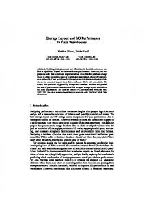
We wanted to explore several issues via simulations. First we wanted to ascertain the ability of the DDM model to identify state functions. Second, we wanted to check whether the hierarchy model improved the performance of the system. Third, we wanted to check how much the model was sensitive to noise. Finally, we wanted to examine whether increasing the number of agents and using better equipped sampling agents improved performance. 4.1 Simulation Environment We developed a simulation of the ANTS domain to test the model. The simulation consists of an area of a fixed size in which Dopplers attempt to identify the object state functions of moving targets. Each target had an initial random location and an initial random velocity of up to 50 km. per hour. Targets leave the area when reaching the boundaries of the zone. Each target that leaves the area causes a new target to appear at the same location with the same velocity in a direction that leads it inwards. Therefore, each target may remain in the area for a random time period. Each Doppler has initial random location and a velocity that is less than 50 km. per hour. When a Doppler gets to the border of the controlled area it bounces back with the same velocity. This ensures an even distribution of Dopplers. Evaluation Methods. We collected the state functions produced by agents during a simulation. We used two evaluation criteria in our simulations: (1) target tracking percentage and (2) average tracking time. We counted a target as tracked if the path identified by the agent satisfied the following: (a) the maximum distance between the calculated location and the real location of the target did not exceed 1 meter, and (b) the maximum difference between the calculated v(t) vector and the real v(t) vector was less than 0.1 meter per second and 0.1 radians in angle. In addition, the identified object state functions could be divided into two categories: (1) Only a single function was associated with a particular target and was chosen to be part of the infoMap. Those functions were assigned a probability of 100% corresponding to the actual object state function. (2) Two possible object state functions based on one viewpoint were associated with a target. Each was assigned a 50% probability of corresponding to the actual function. We will say that one set of agents did better than another if they reached higher tracking percentage and lower tracking time with respect to the 100% functions and the total tracking percentage was at least the same. The averages reported in the graphs below were computed for one hour of simulated time. The target tracking percentage time was calculated by dividing the number of targets that the agents succeeded in tracking, according to the above definitions, by the actual number of targets during the simulated hour. In total, 670 targets passed through the controlled area within an hour in the basic settings experiments described below. The tracking time was defined as the time that the agents needed to find the object state function of the target from the time the target entered the simula-

142


tion. Tracking average time was calculated by dividing the sum of tracking time of the tracked targets by the number of tracked targets. Note that 29% of the targets in our experiments remained in the area less than 60 seconds in our basic settings. Basic Settings. The basic setting for the environment corresponded to an area 1200 by 900 meters. In each experiment, we varied one of the parameters of the environment, keeping the other values of the environment parameters as in the basic settings. The Dopplers were mobile and moved randomly as described above. Each Doppler stopped every 10 seconds, varied its active sensor randomly, and took 10 measurements. The maximum detection range of a Doppler in the basic setting was 200 meters; the number of Dopplers was 20 and the number of targets at a given time point was 30. The DDM hierarchy consisted of only one level. That is, there was one sampler-leader that was responsible for the entire area. We first compared several settings to test the hierarchy model and the sampling agents characterizations. Each setting was characterized by (i) whether we used a hierarchy model (H) or a flat model (F); (ii) whether the sampler-agents were mobile (M) or static (S); and (iii) whether Dopplers varied their active sectors from time to time (V) or used a constant one all the time (C). In the flat model the sampler agents used their local capsules to produce object state functions locally. Mobile and dynamic vs. static Dopplers. In preliminary simulations (not presented here for space reasons) we experimented with all combinations of the parameters (i)-(iii) above. In each setting, keeping the other two variables fixed and varying only the mobility variable, the mobile agents did better than the static ones (with respect to the evaluation definition above). Hierarchy vs. flat models. We examined the characteristics of 4 different settings: (A) FSC that involves static Dopplers with a constant active sector using a nonhierarchical model; (B) HSC as in (A) but using the hierarchical model; (C) FMV with mobile Dopplers that vary their active sectors from time to time, but with no hierarchy; (D) HMV as in (C) but using the hierarchical model. We tested FSC on two experimental arrangements: randomly located Dopplers and Dopplers arranged in a grid formation to achieve better coverage. There was no significant difference between these two FSC formations. Our hypothesis was that the agents in HMV would do better than the agents in all of the other settings.

Figure 3: Target tracking percentage and average time by the settings

The first finding is presented in the left part of Figure 3. This indicates that the setting does not affect the overall tracking percentage (i.e., the tracking percentage of the 50% and 100% functions). The difference between the settings is with respect to the division of the detected target between accurate tracking and mediocre tracking. HMV performed significantly better than the other settings. It found significantly


143

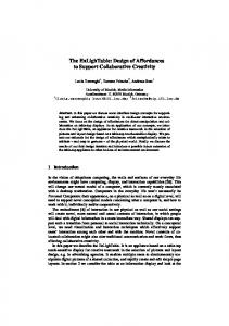
more 100% functions and did it faster than the others. This supports the hypothesis that a hierarchical organization leads to better performance. Further support for a hierarchical organization comes from HSC being significantly better than FMV even though, according to our preliminary results, HSC uses Dopplers that are more primitive than the Dopplers FMV. Another aspect of the performance of the models is the average tracking time as shown in the right part of Figure 3. Once again, one can see that hierarchically based organizations lead to better results. We found that by considering only targets that stayed in the controlled zone at least 60 seconds, HMV reached 87% tracking percentage where 83% were accurately detected We also considered a hierarchy with two levels: one zone leader leading four sampling leaders. The area was divided equally between the four sampling leaders, and each obtained information from the many mobile sampling agents located in its area. In this configuration Dopplers were able to move from one zone to another; Dopplers changed their sampling leader every time they moved from one zone to another. Comparing the results of the two-level hierarchy simulations (not presented here because of space reasons), with the one level hierarchy simulations we found that there was no significant difference in the performance (with respect to the evaluation definition) of the system when there were two levels of the hierarchy when there was only one level in the hierarchy. However, consistent with theorem 1, the computation time of the system was much lower. Communication and noise. While the performance of the hierarchy-based models are significantly better than the non-hierarchy ones, the agents in the hierarchy model must communicate with one another, while no communication is needed for the flat models. Thus, if no communication is possible, then FMV should be used. When communication is possible, however, messages may be lost or corrupted. The data structure exchanged in messages is the capsule. In our simulations using a hierarchy model, each sampling agent transmitted 168 bytes per minute. We examined the influence of randomly corrupted capsules on the HMV’s behavior. Figure 4 shows that as the percentage of the lost capsules increased the number of tracked targets decreased; however, up to a level of 10% noise, the detection percentages decreased only from 74% to 65% and the accurate tracking time increased from 69 seconds to only 80 seconds. Noise of 5% resulted in a smaller decrease to a tracking accuracy of 70% while the tracking time increased slightly to 71. DDM could even mange with noise of 30% and track 39% of targets with average tracking time of 115 seconds. In the rest of the experiments we used the HMV settings without noise. Varying the number of Dopplers and targets. We examined the effect of the number of Dopplers on performance. We found that, when the number of targets was fixed, then as the number of Dopplers increased the percentage of accurate tracking increased as well. The significance of this result is that it confirms that the system can make good use of additional resources. We also found out that as the number of Doppler sensors increased, the 50% probability paths decreased. This may be explained by the fact that 100% paths result from taking into consideration more than one sample viewpoint. We also found that increasing the number of targets, while keeping the

144


number of Dopplers fixed, does not influence the system’s performance. We speculate that this is because an active sector could distinguish more than one target in that sector.

Figure 4: Target detection percentage and average time as function of the communication noise

Figure 5: Tracking percentage and average time as a function of the number of Dopplers

Maximum detection range comparison. We also tested the influence of the detecting sector area on performance. The basic setting uses Dopplers with detection range of 200 meters. We compared the basic setting to similar ones with detection ranges of 50,100 and 150 meters. We found that as the maximum range increased the tracking percentage increased up to the range covering the entire global area. As the maximum radius of detection increased the tracking average time decreased. This is a beneficial property, since it indicates that better equipment will lead to better performance.

5

Conclusions and Related Work

We have introduced a hierarchical approach for combining local and partial information of large-scale object and team environments where agents must identify the changing states of objects. To apply the DDM model to a different environment, it is only necessary to represent three domain-specific functions: PosS, that maps measurements to possible states; ResBy, that determines whether one given object state associated with a time point can be the consequence of another given object state associated with an earlier time point; and pathToFunc, that, given a path, returns a function to represent it. Given these functions, all the DDM algorithms implemented for the ANTS domain are applicable, as long as the complexity of these functions can be kept low. Thus, we believe that the results obtained for the ANTS simulations will carry over to any such domain. The results reported in this paper support the following conclusions: (i) the hierarchy model outperforms a flat one; (ii) the flat mobile dynamic sector setting can be used in situations where communication is not possible; (iii) increasing resources increases performance; (iv) under the identified constraints, it is beneficial to add more levels to the hierarchy; and (v) the DDM can handle situations of noisy communications. In terms of related work, the benefits of hierarchical organizations have been argued by many. So and Durfee draw on contingency theory to examine the benefits of


145

a variety of hierarchical organizations; they discuss a hierarchically organized network monitoring system for object decomposition and also consider organizational self-design [6,7]. DDM differs in its use of organizational structure to dynamically balance computational load. The idea of combining partial local solutions into a more complete global solution goes back to early work on the distributed vehicle monitoring testbed (DVMT) [5]. DVMT also operated in a domain of distributed sensors that tracked objects. However, the algorithms for support of mobile sensors and for the actual specifics of the Doppler sensors themselves is novel to the DDM system. Within the DVMT, Corkill and Lesser [2] investigated various team organizations in terms of interest areas which partitioned problem solving nodes according to roles and communication, but were not initially hierarchically organized [8]. Wagner and Lesser examined the role that knowledge of organizational structure can play in decisions [9]. All the alternative approaches to the ANTS problem (e.g., [4]) have been based on local assessment methods that require coordinated measurements from at least three Doppler sensors and intersecting the resulting arcs of each. Such coordination requires good synchronization of the clocks of the sensors and therefore communication among the Doppler agents to achieve that synchronization. In addition, communication is required for scheduling agent measurements. We have presented alternative methods, which can combine partial and uncertain local information.

References 1. ANTS Program Design Document, unpublished. 2. Corkill, Daniel, and Lesser, Victor. The use of meta-level control for coordination in a distributed problem solving network. In Proceedings of the Eighth International Joint Conference on Artificial Intelligence, pp. 748-756. August, Karlsruhe, Germany, 1983. 3. G. P. Thomas, The Doppler effect, London: Logos, 1965. 4. Leen-Kiat Soh, Costas Tsatsoulis, Reflective Negotiating Agents for Real-Time Multisensor Target Tracking. IJCAI 2001: 1121-1127. 5. Lesser V., Corkill D. and Durfee E., An update on the Distributed Vehicle Monitoring Testbed, CS Technical Report 87-111, University of Massachusetts, Amherst, 1987. 6. So Y., Durfee E., Designing Tree-Structured Organizations for Computational Agents, Computational and Mathematical Organization Theory, 2(3), pages 219-246, 1996. 7. So Y., Durfee E., A Distributed Problem-Solving Infrastructure for Computer Network Management. International Journal of Intelligent and Cooperative Information Systems, 1(2):363-392, 1992. 8. W. Richard Scott, Organizations: Rational, Natural and Open, Prentice-Hall, 1992. 9. Wagner Thomas and Lesser Victor. Relating Quantified Motivations for Organizationally Situated Agents. In Intelligent Agents VI --- Proceedings of the Sixth International Workshop on Agent Theories, Architectures, and Languages, Lecture Notes in Artificial Intelligence, pp. 334-348. April, 1999.