Jan 1, 2018 - We will reconsider the ABCD law of ray beam propagation within the context ...... In theoretical biology the Kleiber law links the metabolic power ...
LECTURES ON MATHEMATICAL METHODS FOR PHYSICS D. BABUSCI INFN - Laboratori Nazionali di Frascati Via E. Fermi 40, 00044 Frascati, Roma G. DATTOLI ENEA - Unità Tecnica Sviluppo di Applicazioni delle Radiazioni Laboratorio di Modellistica Matematica Centro Ricerche Frascati, Roma M. DEL FRANCO ENEA Guest
RT/2010/58/ENEA
AGENZIA NAZIONALE PER LE NUOVE TECNOLOGIE, LʼENERGIA E LO SVILUPPO ECONOMICO SOSTENIBILE
LECTURES ON MATHEMATICAL METHODS FOR PHYSICS D. BABUSCI INFN - Laboratori Nazionali di Frascati Via E. Fermi 40, 00044 Frascati, Roma G. DATTOLI ENEA - Unità Tecnica Sviluppo di Applicazioni delle Radiazioni Laboratorio di Modellistica Matematica Centro Ricerche Frascati, Roma M. DEL FRANCO ENEA Guest
RT/2010/58/ENEA
I Rapporti tecnici sono scaricabili in formato pdf dal sito web ENEA alla pagina http://www.enea.it/produzione_scientifica/edizioni_tipo/Rapporti_Tecnici.html This report has been prepared and distributed by: Servizio Edizioni Scientifiche ENEA - Centro Ricerche Frascati, C.P. 65 - 00044 Frascati, Rome, Italy I contenuti tecnico-scientifici dei rapporti tecnici dell'ENEA rispecchiano l'opinione degli autori e non necessariamente quella dell'Agenzia. The technical and scientific contents of these reports express the opinion of the authors but not necessarily the opinion of ENEA.
LECTURES ON MATHEMATICAL METHODS FOR PHYSICS D. BABUSCI, G. DATTOLI, M. DEL FRANCO
Abstract This book is devoted to the presentation of a series of lectures on mathematical methods for Physics. It has been planned for graduate students and treats different topics, going from classical optics to relativistic quantum mechanics, using a common thread which is mainly based on operators and their properties. Extensive use of special functions in physical applications is presented with particular emphasis on their usefulness in the solution of ordinary and partial differential equations. Key words: Operators, special functions, quantum mechanics, relativistic theories, ordinary and partial differential equations Riassunto In questo libro sono presentate una serie di lezioni sui metodi matematici per la Fisica. E’ stato pensato per studenti laureati e tratta diversi argomenti, dall’ottica classica alla meccanica quantistica relativistica, seguendo un approccio prevalentemente basato sugli operatori e le loro proprietà. E’ trattato il ruolo delle funzioni speciali nelle varie applicazioni fisiche, con particolare attenzione alla loro utilità nella soluzione di equazioni differenziali ordinarie e parziali. Parole chiavi: Operatori, funzioni speciali, meccanica quantistica, teorie relativistiche, equazioni differenziali ordinarie e alle derivate parziali
5
SUMMARY 1. 1.1. 1.2. 1.3. 1.4. 1.5. 1.6. 1.7. 1.8. 2.
2.1. 2.2. 2.3. 2.4. 2.5. 2.6. 2.7. 3. 3.1. 3.2. 3.3. 3.4. 3.5. 3.6. 3.7. 3.8. 3.9. 4. 4.1. 4.2. 4.3. 4.4. 4.5. 4.6. 4.7.
CHAPTER I MATRICES, EXPONENTIAL OPERATORS AND THEIR APPLICATIONS TO PHYSICAL PROBLEMS Introduction The Pauli Matrices Some examples of applications of matrices from classical optics: ray beam propagation and ABCD law. Some examples of applications from quantum mechanics Examples from particle physics: Kaon mixing Cabibbo Angle and the Seesaw mechanism The Gell Mann matrices as generalization of the Pauli matrices Concluding remarks
19 27 30 37 41 50
CHAPTER II ORDINARY AND PARTIAL DIFFERENTIAL EQUATIONS, THE EVOLUTION OPERATOR METHOD AND APPLICATIONS TO PHYSICAL PROBLEMS Ordinary differential equations, matrices and exponential operators Partial differential equations and exponential operators, I Partial differential equations and exponential operators, II Operator ordering The Schrödinger equation and the Paraxial wave equation of classical optics Examples of Fokker-Planck, Schrödinger and Liouville equations. Concluding Remarks
65 68 73 74 80 86 89
CHAPTER III THE HERMITE POLYNOMIALS AND THEIR APPLICATIONS Introduction The generating function of Hermite polynomials The Hermite polynomials as an orthogonal basis Hermite polynomials in quantum mechanics: creation and annihilation operators. Applications to some quantum mechanical problems Coherent or quasi-classical states of harmonic oscillators The Jaynes-Cummings model Classical Optics and Hermite polynomials Concluding Remarks
97 100 104 108 111 115 120 122 123
CHAPTER IV THE LAGUERRE POLYNOMIALS, INTEGRAL OPERATORS AND THEIR APPLICATIONS Introduction The generating Functions of Laguerre polynomials The orthogonality properties of the Laguerre polynomials Bessel functions The associated Laguerre polynomials The Legendre polynomials Concluding remarks
129 132 133 136 140 142 143
9 13
6
5. 5.1. 5.2. 5.3. 5.4. 5.5. 5.6. 5.7. 5.8. 6. 6.1. 6.2. 6.3. 6.4. 6.5. 6.6. 6.7. 7. 7.1. 7.2. 7.3. 7.4. 7.5. 7.6. 7.7. 8. 8.1. 8.2. 8.3. 8.4. 8.5. 8.6.
CHAPTER V EXERCISES AND COMPLEMENTS I Pauli and Jones Matrices and Mueller calculus The Dirac Matrices, Quaternions and higher order respesentation of th56 Spin Matrices Matrix equations The Lorentz Transformation Hyperbolic trigonometry and special relativity Elliptic Functions The Mathematics of the Higgs mechanism A Formal point of view to the dimensions and units in Physics
156 164 166 169 174 176 187
CHAPTER VI EXERCISES AND COMPLEMENTS II Ordinary differential equations and matrices Gamma Function and Definite Integrals Complex variable method and evaluation of integrals Crofton-Gleisher identities and heat type equations Fourier transform Fourier transform and the solution of differential equations Fourier-type transforms
197 208 215 220 224 234 237
CHAPTER VII EXERCISES AND COMPLEMENTS III The second solution of the Hermite equation Higher orders Hermite polynomials Multi-index Hermite polynomials On the algebra of Creation-Annihilation operators and some physical applications The Eisenstein Integers Comments on some formal aspects of the Harmonic Oscillator Hamiltonian and further miscellaneous considerations Time-dependent Hamiltonians CHAPTER VIII EXERCISE AND COMPLEMENTS IV The Sturm Liouville problem The Green’s Functions Laguerre Polynomials, associated operators and partial differential equations Appèl Polynomials, associated operators and partial differential equations The Riemann Function Bessel Functions
149
243 245 250 252 257 263 265
269 273 275 280 285 291
7
FOREWARD We report in the following a collection of lectures on Mathematical Methods of Physics and, in planning the topics to be discussed, the first problem we have been faced with has been the question “Which methods for which Physics?” Our goal was not that of providing a series of lectures on well known problems in Mathematical Physics, but rather to give some tools to attack specific problems, which are often encountered in different branches of Physics, ranging from quantum field theory, to laser Physics and to charged particle transport in accelerators. The power of Mathematics, or better what has been called its unreasonable success in describing physical phenomena, is just the fact that the same formalism can be exploited to model different aspects of Physics. The formalism of matrices is useful in quantum mechanics to study the dynamical behavior of particles with spin, but it turns out to be useful to study the propagation of optical beams through lens systems or to treat the charged beam transport in Linacs or in Storage Rings. The Schrödinger equation can be used to study the quantum mechanical spreading of a free particle and the distribution of electromagnetic fields in an optical cavity as well, the heat equation can be exploited in so a large number of contexts, which even include the behavior of the stock options in the financial markets. Our choice has been therefore that of picking up a certain number of mathematical techniques, of discussing them carefully and also to present the physical problems to which they apply. We have therefore touched problems in classical and quantum electromagnetism, in particle and solid state Physics, by taking always into account a kind of unitarity (at least formal) between the different physical phenomena. This is an attempt which requires some effort by the reader, since we have not used sharp cuts between quantum and classical mechanics or between high energy and solid state Physics, we have mainly been guided by the evolution and by the internal mathematical consistency of ideas flowing from matrices, to differential operators, to group theory… We owe our gratitude to Prof. O. Ragnisco and to Prof. Decio Levi who allowed this experiment and encouraged and advised us during the preparation of the lectures.
8
“If you intend to mount heavy mathematical artillery again during your coming year in Europe, I would ask you not only not to come to Leiden, but if possible not even to Holland, and just because I am really so fond of you and want to keep it that way. But if, on the contrary, you want to spend at least your first few months patiently, comfortably, and joyfully in discussions that keep coming back to the same few points, chatting about a few basic questions with me and our young people- and without thinking much about publishing- then I welcome you with open arms!! ". (Eherenfest in a letter to Oppenheimer, Summer 1928)
9
1. CHAPTER I MATRICES, EXPONENTIAL OPERATORS AND THEIR APPLICATIONS TO PHYSICAL PROBLEMS 1.1.
Introduction
The matrices and the relevant formalism are widely exploited tools in Physics and Mathematics. They provide, indeed, the back bone of the treatment of many problems in classical and quantum Physics. We start, therefore, these lectures with a short resume on the properties of matrices, aimed at fixing the notation and illustrate the technicalities we will later employ in solving mathematical problems of physical interest. Our starting point is the equation1 Aˆ x b
(1.1.1)
where 11 1 2 , Aˆ 2 1 2 2
,
ij
, ,
(1.1.2)
Aˆ is therefore a 2 2 matrix and the other quantity denotes a column vector.
Eq. (1.1) can be considered the generalization of an algebraic equation of first degree (it represents indeed an algebraic system of first order equations), and, provided that we accept the matrix as the generalization of the ordinary numbers, its solution can, therefore, be written in the form x Aˆ 1 b
(1.1.3)
reminiscent of the solution of first degree algebraic equations. Such a formal solution makes sense if the matrix Aˆ is not singular, or, what is the same, if it is invertible. It goes by itself that, in deriving eq. (1.1.3), we have tacitly assumed that Aˆ Aˆ 1 1ˆ
The symbol Oˆ will denote either a matrix or an operator, the column vectors will be denoted by specified by any extra symbol. 1
(1.1.4)
, the scalars will not be
10
where we have denoted with 1 0 1ˆ 0 1
(1.1.5)
the real-unity matrix, satisfying the obvious property 1ˆ Bˆ Bˆ 1ˆ Bˆ ,
1ˆ ,
(1.1.6)
valid for any generic 2 2 matrix. It is easily checked that the inverse of Aˆ writes 1 22 Aˆ 1 21
1 2 , 11
(1.1.7)
where is the matrix determinant 11 2 1 1 2 21 .
A matrix will be said singular, and thus not invertible, if its determinant is vanishing. Needless to say we have just “rediscovered” the well known solution of a system of first order algebraic equation with the Cramer’s method, using a point of view aimed at showing that, within certain limits, we can use matrices as suitable generalizations of the ordinary numbers (complex or real). We can therefore define simple procedures to introduce operations like sum, difference, product and power. As a further support to the previous statements, let us note that, along with the matrix (1.1.5), playing the role of unity, we can introduce the matrix 0 1 iˆ 1 0
(1.1.8)
called the imaginary matrix (or sympletic unit), which plays the role of the imaginary unity matrix, since iˆ 2 1ˆ .
(1.1.9)
We can make a further step in the direction of considering matrices as ordinary numbers, by introducing the notion of a function of a matrix. Accordingly we will say that Fˆ f ( Aˆ )
(1.1.10a)
11
is a matrix, which is explicitly defined through the Taylor series expansion of the function f(x), namely f ( n ) (0) ˆ n f ( Aˆ ) A , n! n0
(1.1.10b)
with f (n ) (0) denoting the n-th derivative calculated at x=0. The above expansion is just a formal expression, since we did not specify any radius of convergence, which, on the other side, cannot be stated in abstract terms from the expansion itself. The convergence can be checked a posteriori, using, for example, the following procedure. By considering the matrix operator Fˆ acting on a generic column vector , we have: f Fˆ n0
(n)
(0) ˆ n f ( n ) ( 0) f ( n ) (0) ˆ n (A ) A n! n! n! n0 n 0
n
n
Aˆ n ,
(1.1.10c)
and all the operation is meaningful if the last series in (1.1.10c) is convergent, i.e. the definition of the function of a matrix holds only if the function admits a series expansion, as in the case of analytical functions. We will show, with a simple example, where (1.1.10b) may lead, by considering the following exponentiation of the imaginary matrix e
iˆ
n 0
n ˆn
(1) n 2 n ˆ (1) n 2 n 1 ˆ i 1 i cos 1 sin iˆ. n! (2 n)! n 0 n 0 ( 2 n 1)!
(1.1.11)
The use of the correspondences 1 1ˆ,
i iˆ,
(1.1.12)
suggest that eq. (1.1.11) is a generalization of the Euler formula, involving the imaginary unit matrix instead of the imaginary unit. Written in a matrix form, eq. (1.1.11) yields cos ˆ e i Rˆ ( ) sin
sin . cos
(1.1.13)
We can therefore state that the exponentiation of the imaginary matrix leads to the
two dimensional rotation matrix.
The matrices are generalizations of the ordinary numbers and they have therefore more general properties which will be discussed below. Let us now consider the 2 2 matrix
12
0 1 hˆ , 1 0
(1.1.14)
which will be defined the hyperbolic unit matrix. It is, indeed, easily checked that it satisfies the following relation, hˆ 2 1ˆ ,
(1.1.15a)
and that its exponentiation yields cosh ˆ e h Rˆ h ( ) sinh
sinh . cosh
(1.1.15b)
Note that the matrix (1.15b) represents a rotation in a hyperbolic space (hence the name hyperbolic of the unit hˆ ) and its mathematical and physical meaning will be more deeply discussed in the following. Unlike ordinary numbers matrices are not commuting entities. We may, therefore, expect that the three units: 1ˆ, iˆ, hˆ do not commute. It is easily checked that the real unit matrix commutes, by definition, with any matrix, while the imaginary and hyperbolic units yield
iˆ, hˆ iˆ hˆ hˆ iˆ 2 tˆ,
1 0 . tˆ 0 1
(1.1.16)
The matrix tˆ is a fourth unit and satisfies the conditions tˆ 2 1ˆ,
e ˆ e t Sˆ ( ) 0
0 . e
(1.1.17)
The matrix Sˆ ( ) is called the squeezing mapping. Its role in physical problems is of paramount importance and will be discussed later. The four matrices iˆ, hˆ, tˆ, 1ˆ represent the basis to express any 2 2 matrix. We have indeed 11 12 1ˆ iˆ hˆ tˆ , 22 21
(1.1.18)
where , , , are the coefficients of the linear combination and can be expressed in terms of the matrix entries. If we limit our analysis to traceless matrices only, i.e. it is zero the sum of the elements of the principal diagonal
13
11 22 0
(1.1.19)
we can trace out the real unity matrix and use as basis the remaining units. Before concluding this section, let us remind that we can define the hermitian conjugate of the matrix Aˆ as * * ˆA 11 21 , * * 22 12
(1.1.20)
and, therefore, we find that the simplectic unit is anti-hermitian, namely iˆ iˆ,
(1.1.21)
while all the other matrices are Hermitian.
1.2.
The Pauli Matrices
In the previous section we have introduced a set of matrices and we have shown that at least two of them, once exponentiated, generate rotations of circular or hyperbolic nature. Concerning the circular case, we have stressed that the operation x cos sin x ˆ e i y sin cos y
(1.2.1a)
generates the rotation of the plane coordinates x, y. This conclusion, even though
apparently trivial, is extremely interesting, and opens the way to further speculations about the notion of Lie Group, which will be discussed later touched on in these lectures. By keeping the derivative of both sides with respect to , we find d d
iˆ
(1.2.1b)
Furthermore if we set iˆ ˆ ˆ ,
with
(1.2.2)
14
0 1
0 0
ˆ , ˆ 0 0 1 0
(1.2.3)
satisfying the identity ˆ 2 0ˆ ( with 0ˆ being the null matrix, i.e. a matrix with all vanishing entries), we can recast eq. (1.2.1b) in the form d d
ˆ ˆ .
(1.2.4)
This is essentially the Schrödinger equation with the Hamiltonian Hˆ i (ˆ ˆ ).
(1.2.5)
The Hermiticity of Hˆ ensured by the fact that the operators (1.2.3) satisfies also the identitiy ˆ ˆ .
(1.2.6)
As we will see in the forthcoming parts of this chapter, the Hamiltonian (1.2.5) is a paradigmatic tool for the study of two-level quantum mechanical systems, but, before discussing these aspects of the problem, some naïve algebraic manipulations are in order. We first note that the above matrices are not commuting, we get indeed
ˆ , ˆ 2 ˆ 3 , 1 1 ˆ 2 0 , ˆ 3 t 2 0 1 2 ˆ 3 , ˆ ˆ ,
(1.2.7)
which are equivalent to the commutation relations of the angular momentum operator components in quantum mechanics By using the language of the theory of groups, we can say that these matrices realize one of the representations of the generators of the uni-modular group SU (2) 2 . The matrices ˆ , ˆ 3 are the Pauli matrices 3 , introduced during the pioneering days of quantum mechanics to describe the spin dynamics. The solution of the previous Schrödinger problem can be written in the form ( ) Uˆ ( ) 0
In a following chapter of these lectures we will discuss different realizations of the familiar case employing differential operators. 2
3
Strictly speaking, the Pauli matrices are ˆ1 hˆ, ˆ 2 i iˆ, ˆ 3 tˆ.
(1.2.8a)
SU (2) group including the more
15
where the operator Uˆ ( ) e (ˆ ˆ )
(1.2.8b)
denotes the evolution operator, associated with the solution of eq. (1.2.4), which, from the mathematical point of view, is an initial value Cauchy problem. The unitarity4 of the Uˆ operator is easily checked and follows from the hermiticity of the operator (2.5). The argument of the exponential in (2.8b) contains two matrices which are not commuting quantities. It is therefore evident that this imposes some cautions in handling the so called disentanglement of the above exponential as a product of exponential operators; we have indeed that, as an obvious consequence non commutative character of the matrices, the “semi group” property5 of the exponential e a e b e b e a e a b
(1.2.9)
does not hold anymore, and e (ˆ ˆ ) e ˆ e ˆ e ˆ e ˆ .
(1.2.10)
This fact implies that we must take into account appropriate ordering criteria!!! The problems underlying operator ordering play a central role in modern theoretical Physics and will carefully be treated in these lectures. Here we use a simple, but effective, argument, which can be easily generalized. We assume that a convenient ordering for the previous exponential operator is a product of three exponential operators, containing the group generators, namely e (ˆ ˆ ) e 2 h ( )ˆ 3 e f ( )ˆ e g ( )ˆ
,
(1.2.11a)
where the functions h( ), f ( ), g ( ) are the characteristic ordering functions, satisfying the “initial” condition (1.2.11b)
h(0) f (0) g (0) 0.
To proceed further, we note that, as a consequence of eqs. (1.10.b), (1.1.17) and (1.2.6) we have 1 e f ( ) ˆ 0 4
f ( ) 0 e h ( ) 1 , e g ( ) ˆ , e 2 h ( )ˆ 3 1 g ( ) 1 0
0 e h ( )
(1.2.13)
We remind that an operator is said unitary if its hermitian conjugate is equal to its inverse. From eq. (1.2.8b) we get indeed
Uˆ ( ) e (ˆ ˆ ) e (ˆ ˆ ) Uˆ 1 ( ) .
5
In mathematics a semigroup is an algebraic structure consisting of a set closed under a binary associative operation.
16
and therefore the products of the previous matrices yields e
2 h ( )ˆ 3
e
f ( ) ˆ
e
g ( )ˆ
e h ( ) 0
e h ( ) (1 g ( ) f ( )) g ( ) e h ( )
0 1 e h ( ) 0
0 f ( ) 1 1 g ( ) 1
(1.2.14)
f ( ) e h ( ) . e h ( )
The reader can verify that the above matrix has unit determinant. Its unitarity is a consequence of the fact that the operator ˆ ˆ is anti-Hermitian6. Furthermore, because ˆ ˆ iˆ
(1.2.15)
we know that the overall effect of the evolution operator is that of producing a rotation, which can always be decomposed in three successive distinct actions, generated by the exponential operators. We will discuss the physical meaning of the previous result in the forthcoming sections; here we note that by comparing eq. (1.2.14) with the rotation matrix we can specify the characteristic functions as follows (why?) e h ( ) sec ,
1 f ( ) sin 2 , g ( ) tan . 2
(1.2.16)
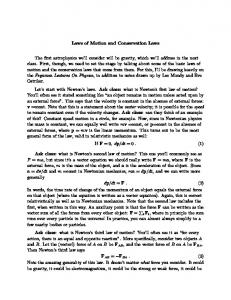
In Fig. (1.2-1) we have reported a “geometric” interpretation of the characteristic functions, which are related to a kind of decomposition of the ordinary rotation matrix. Further comments on such “interpretation” can be found in the second part of these lectures (chapter 5, sec. 5).
g (α) α f (α)
α
eh(α) Fig. 1.2-1 Characteristic functions g ( ), f ( ) and e h ( ) 6
The reader can also prove that the unitarity condition imposes that
1 1 g ( ). f ( ) g ( )
17
The previous results are relevant to the particular case, in which the matrix in the argument of the exponential contains non diagonal entries only. We will treat a more general situation in which the matrix is anti-hermitian (why?) and with vanishing trace. To this aim we introduce the following operator written in vector form
(ˆ x , ˆ y , ˆ z ), 1 0 1 2 1 0 1 10 ˆ y (ˆ ˆ ) 2i 2i 1 1 2
ˆ x (ˆ ˆ )
(1.2.17)
1 0
1 1 0 . 2 0 1
ˆ z ˆ 3
The vector components satisfy the relations of commutation of angular momentum
ˆ , ˆ i j
k
ˆ l ,
j, k,l
( j , k , l x, y , z )
(1.2.18)
where jk l is the Levi Civita tensor. The use of such an operator allows the definition of the following Hamiltonian operator Hˆ n ,
n ,
(1.2.19)
where is the modulus of the vector , usually called the torque vector, and n is the unit vector defining its direction. The physical meaning of the previous Hamiltonian will be discussed in the forthcoming sections. The associated evolution operator writes ( Uˆ e
i
Hˆ t
)
Uˆ (t ) e i t n
(1.2.20)
and the reader will not find any problem in proving that t t Uˆ (t ) cos( ) 1ˆ 2i sin( ) n 2 2
(1.2.21)
1 (hint: note that n 2 1ˆ and use the same procedure leading to eq. (1.1.11)). 4
Before concluding this section we want to stress the following points
18
a) An exponential operator containing a 2 2 matrix (with vanishing trace) can always be written as the ordered product of three exponentials containing the Pauli matrices, like in eq. (1.2.11a)7
Uˆ (t ) ei ˆ 3 t (ˆ ˆ ) e 2 h ( ) ˆ 3 e f ( ) ˆ e g ( ) ˆ ;
(1.2.22)
b) The ordering (1.2.11a) is valid for the exponentiation of any linear combination of the angular momentum operators and is independent of the specific representation (this aspect of the problem will be discussed in the forthcoming Chapters). The reader may prove his degree of understanding of the topics discussed in these sections by considering the problems proposed below. The operator ordering in eq. (1.2.11a) is one of the 3! possible ordered forms, it goes by itself that each form will be characterized by an appropriate set of characteristic functions as e. g. Uˆ ( ) e ( ) ˆ e ( ) ˆ e 2 ( ) ˆ 3 .
(1.2.23)
We invite the reader to find the link between the different characteristic functions, corresponding to different exponential ordering. The proof of the following identity
i ,
(1.2.24)
and the understanding of its physical and geometric meaning is an important exercise. (hint: use the ordinary definition of the vector product and then the commutation relations (2.7)).
Finally, given a generic (2x2) matrix with trace 0 , the reader is invited to prove that e
11 12 21 2 2
A11 A21
A12 A22
where:
7
The evolution operator is associated with a Hamiltonian operator Hˆ ˆ 3 i ˆ ˆ
(1.2.25)
19
1 1 2 Tr (ˆ ) (11 2 2 ) sinh( ) cosh( )e , A11 2 2 1 1 2 Tr (ˆ ) (11 2 2 ) sinh( ) cosh( )e , A2 2 2 2 12 Tr (ˆ ) A12 A21 2 sinh( )e , 1 2 21 2 (11 22 ) 2 4 1 2 21. Tr (ˆ ) 11 2 2 ,
(1.2.26)
(hint: Take into account that the matrix at the exponent is not traceless, therefore it writes as a combination of Pauli matrices including the unit matrix…) Here we have introduced and discussed the properties of 2 2 matrices useful to describe two-level systems or spin doublets (or ½ spin particles). The case of three level systems or spin 1 particles (spin triplets) requires the use of 3 3 matrices, as it will be briefly discussed in the next sections and more carefully in Chapter 5. The results obtained in this section will provide the mathematical apparatus for treating the physical problems we will discuss in the forthcoming sections.
1.3. Some examples of applications of 2 2 matrices from classical optics: ray beam propagation and ABCD law. Talking about Pauli matrices, the most natural application coming to mind is the dynamics of particles with
1 spin in a magnetic field. This problem will be discussed in 2
the following section. Here we show how the Pauli matrices can be used to discuss other physical problems, usually not treated within these frameworks. In Fig. 1.3-1 we have reported the transmission of optical beams through an etalon, which can be considered as an interface of thickness l between media with different optical indices. This process is usually described using elementary mathematical tools, however the propagation of optical beams through such optical systems can be conveniently described using the matrix formalism, which may provide, as we will see below, a significant improvement.
20
n θ
T1
R1
T2
R2 l
Fig. 1.3-1 Optical ray beams reflected and transmitted through an etalon
The direction of propagation inside the etalon is that parallel to the straight lines perpendicular to its surface. The axis of propagation is that passing through its middle plane. The ray position and angles (see Figs. 1.3-2,3) are defined with respect to the optical axis and here we limit ourselves to the case of paraxial propagation, i.e. ray propagation involving small angular deviation from the propagation axis. If we characterize the ray beam in terms of a column vector having as components its distance from the optical axis and the angle it forms with the axis direction, the problem of the ray propagation 8 , whatever complicated the optical system is, can always be reduced to that of finding the relationship between input and output rays, in terms of the following relation A B r r 0 C D i
(1.3.1)
where the matrix with entries A, B, C, D is said the transport matrix and characterizes the optical element (or the combination of a series of optical elements) guiding the beam.
8
Along with propagation we will use as “synonyms” evolution and transport.
21
n=n3
n=n1
n=n2
Example optical system
θ Input
d2 2 d1
r
3
d3 R
f d4
4
n=n4 5 d 5
Curved interface
6
d6
Flat interface
Flat interface
Flat interface Thin lens
d7
r' 8
θ'
Output 7
Flat mirror
Fig. 1.3-2 Input and output ray-beams from a complicated optical system. The dotted line represents the propagation axis and position and angles are taken with respect to it as indicated in the figure.
The simplest optical transport element is the transport matrix is specified by A 1,
B d,
C 0,
free space (see Fig. (1.3-3)), whose
D 1
(1.3.2)
an analogous result can be obtained for a thin lens system, see Fig. (1.3- 4) A 1,
B 0,
C
1 , f
D 1
(1.3.3)
where f is the focal length and the sign specifies the focusing or defocusing nature of the lens, respectively.
22
Derivation of transfer matrix for light propagation in free space ∴ tan( ) = h
d h = d•tan( ) r'= r + d•tan( )
∴ r'= r + d• θ'=θ 1d r' = ' 01
θ'
(using the paraxial approximation than tan(θ) ≈ θ)
r h
Transfer matrix for propagation in free space
r'
θ
d
r
r
Reference axis
Fig. 1.3-3 Ray propagation trough a drift section. d f
Axis Focal point
R1
R2
Positive (converging) lens
Fig. 1.3-4 Ray propagation through a converging lens.
It is now worth noting that, indicating with Oˆ , Fˆ , Dˆ the matrices corresponding to a straight section, a focusing and a defocusing lens, respectively (see Fig. 1.3- 5), Ray propagation d f
Axis Focal point R1
R2 D
F
O
Fig. 1.3-5 Symbols for straight section, focusing and defocusing lens, respectively
23
we have 1 d ˆ 1 d ˆ e d ˆ Oˆ 0 1 1 1 0 ˆ 1 f ˆ ˆ 1 F 1 1 f ˆ e f 1 1 0 ˆ 1 f ˆ ˆ 1 ˆ D e 1 1 f f
(1.3.4)
(hint: see eq. (1.2.3)). The above relations are of noticeable importance since they state that the propagation through optical systems can be accomplished using the formalism of the Pauli matrices and their algebraic properties. We can derive, from the previous equation and according to the discussion of the previous sections, the following identity
Fˆ , Oˆ Fˆ Oˆ Oˆ Fˆ 2 df ˆ , 3
(1.3.5)
d Dˆ , Oˆ 2 ˆ 3 , f
whose physical meaning is clear: it states indeed that the sequence of the optical elements, along a transport line, is important. Even though trivial, such a remark may be helpful in understanding the role of operators in the description of physical devices. We may ask whether the operator Sˆ e bˆ (the already introduced squeeze mapping, see eq.(1.1.17)) can be interpreted as an optical element. To this aim we note that 3
r eb r r eb ˆ 3 b . i e i 0
(1.3.6)
We can conclude that it represents the action of a beam expander, whose practical realization is shown in Fig. (1. 3- 6).
24
f 2 - f1
Axis -f1 R2
R1 f2
Positive (converging) lens
Fig. 1.3-6 Beam expander (Galilean telescope); note that the length of the free region between defocusing and focusing length is f 2 f 1 .
According to the above picture the action of a certain number of successive optical elements is given by the product of a corresponding number of matrices. The successive action of a drift section, a thin focusing lens and a beam expender, can therefore be written as Oˆ Fˆ Eˆ e d ˆ e
1 ˆ f
eb 3
(1.3.7)
which has the same structure of the evolution operator discussed in the previous section and may be exploited to provide a possible physical interpretation of the characteristic functions. The use of the above few elements about the operatorial treatment of optical systems allows some interesting conclusions, which are left as an exercise to the reader a) Prove that the action of two consecutive focusing thin lenses is equivalent to a single thin lens with focal length f
f1 f 2 . f1 f 2
(1.3.8)
b) Consider an optical system composed by a thin lens followed by a straight section. Prove that such a system is equivalent to the following composition 1 ˆ M1 1 f
01 d 1 1 1 0 1 f
d d 1 . f
(1.3.9)
Show that an optical system composed by a drift followed by a thin lens is equivalent to
25
1 d 11 Mˆ 2 0 1 f
d 0 1 f 1 1 f
d Mˆ 1 1
(1.3.10)
Concerning this result it is worth stressing that from the mathematical point of view it is just a consequence of the non-commutativity of the matrices. We invite the reader to consider carefully its physical meaning. c) Show that the Dˆ Oˆ Fˆ of Fig. (1.3-6) corresponds to a beam expander with f b ln 1 . f2
d) Discuss the arrangement Dˆ Oˆ Fˆ and find the condition to obtain a beam reducer. Finally we invite the reader to develop physical arguments to justify the matrices describing the optical elements reported in Tab. (1.3-1) and use the various elements to find the matrix corresponding to the optical element reported in Fig. (1.3- 2). Element
Matrix
Propagation in free space or in a medium of constant refractive index
1 d 0 1
Refraction at a flat interface
1 0
Refraction at a curved interface
Reflection from a flat mirror
1 n1 n2 Rn2
0 n1 n2
Remarks d = distance n1 = initial refractive index n2 = final refractive index.
R = radius of curvature, R > 0 for convex (centre of 0 curvature after interface) n1 n2 n1 = initial refractive index n2 = final refractive index.
1 0 0 1
Identity matrix
Reflection from a curved mirror
1 2 R
0 1
R = radius of curvature, R > 0 for concave
Thin lens
1 1 f
0 1
f = focal length of lens where f > 0 for convex/positive (converging) lens. Valid if and only if the focal length is much greater than the thickness of the lens.
Tab. 1.3-1 Optical element and corresponding ABCD matrix.
26
We will reconsider the ABCD law of ray beam propagation within the context of wave optics in the next chapters. The same formalism can furthermore be applied to circuit network like two-port systems of the type shown in Fig. (1.3-7).
I1
I2
U1
Z11
Z22
Z12
Z21
U2
Fig. 1.3-7 Two port system.
In this case the ABCD law (represented by the impedances Z) connects voltages U and currents I and the reader should not have any problem to find a physical justification for the characterization, reported in Tab. (1. 3-2), of circuit elements in terms of matrices.
Element
Matrix
Remarks
Series resistor
1 R R = resistance 0 1
Shunt resistor
1 1 R
0 1 R = resistance
1 1 Series conductor G G = conductance 0 1 1 0 G = conductance Shunt conductor G 1 Series inductor
1 Ls L = inductance 0 1 s = complex angular frequency
Shunt capacitor
1 Cs
0 C = capacitance 1 s = complex angular frequency
Tab. 1.3-2 Circuit element and corresponding ABCD matrix.
27
1.4.
Some examples of applications from quantum mechanics
In this section we will discuss the use of 2 2 matrix operators in quantum mechanical problems like the dynamics of charged particles with spin interacting with an external magnetic field. The non relativistic Pauli equation describing the coupling of a spin ½ charged particle with an external static magnetic field B writes9 i t q
B 2m
(1.4.1)
where q is the particle charge, m its mass, and is a two-component wave function. Spin up
Fig. 1.4-1 Total spin direction not aligned with Fig. 1. 4. 1any component ( S s( s 1)
3 ) . 2
In Fig. (1.4-1) we have reported a generic spin orientation and if we assume that B is along the y direction, eq. (1.4.1) can be written as t c (ˆ ˆ ) ,
c
qB 4m
(1.4.2)
where c is the cyclotron frequency. According to the discussion of the previous section, the solution of eq. (1.4.2) is almost straightforward, and we get Rˆ ( c t ) 0
(1.4.3)
The equation has been written in the above form by neglecting the kinetic term and by retaining the Stern and Gerlach interaction (magnetic moment – magnetic field) only.
9
28
where Rˆ is the rotation matrix (see eq. (1.1.13)), corresponding to the evolution operator associated with the Hamiltonian the Schrödinger equation (1.4.2). A more general result can be achieved by casting the above equation, in the form t 2iq c n ,
B n B
(1.4.4)
whose solution is again obtained in the form of a rotation. Let us now consider a two level quantum system which will be defined as a quantum system with only two allowed energy states, like an atomic or molecular system. The two states are coupled by some external field, which, in the example of the figure (1.4-2), is an electromagnetic interaction. The Schrödinger equation, accounting for the evolution of such a system, is10 i t ( Hˆ 0 Vˆ )
(1.4.5)
where V is the interaction potential, between upper and lower levels and Hˆ 0 is the unperturbed part of the Hamiltonian, satisfying the eigenvalues equation Hˆ 0 E ,
1 E 2
(1.4.6)
with denoting the wave functions of the two states independent and orthogonal11, and E the relevant energy eigenvalues. The evolution of such a system is ruled by the Schrödinger eq. (1.4.5), and can be written as follows a (t ) a (t )
(1.4.7)
By definition the operator V connects lower and upper levels and does not contain diagonal elements. The equation of motion satisfied by the time dependent coefficients in eq. (1.4.7) can be inferred from the Schrödinger equation and the reader can easily verify that they can be cast in the form
We assume that V can be considered independent of time in the sense that its possible variation with time are very slow compared with the dynamics associated with frequency c . 11 The concept of orthogonal states will be more carefully discussed in the following. Here orthogonal means that 10
*
dV 0 .
29
Before
Atom in excited state
During
After emission
Before
E2 photon hν
Atom in excited state
During
Incident photon hν
After emission E2 photon hν photon hν
E Atom in ground state 1
a)
E Atom in ground state 1
b)
Fig. 1.4-2 A schematic representation of an atomic or molecular two level system coupled by an electromagnetic field.
i t ˆ z 2 ˆ y
(1.4.8)
where a , a
i Vˆ Vˆ .
(1.4.9)
The evolution operator associated with the solution of eq. (1.4.8) is given by eq. (1.2.20) where Uˆ (t ) e i t ,
(0, 2, ).
(1.4.10)
A straightforward application of eq. (1.2.21) leads to the following time dependence of the evolution matrix (why?) t sin( ) t 2 cos i 2 Uˆ (t ) t 2 sin( ) 2
. t sin( ) t 2 cos( ) i 2
t 2 sin( ) 2
(1.4.11)
The probability that the two level system will be found in the state is therefore given by P (t )
where
2
2
2 t t 2 cos( ) a 0 2 sin(t ) a 0 2 sin( ) 2 a 0 2 2
(1.4.12)
30
a 0 a 0 a t a t 1. 2
2
2
2
(1.4.13)
The concept of two level system is a kind of abstraction which applies to a large variety of problems in Physics. Apart from the example referring to atomic or molecular systems, one should quote the so called isotopic doublets, in which the isotopic spin is used to treat, as we will see below, the neutron and the proton as different manifestation of a unique particle, the nucleon. The examples discussed in the forthcoming sections clarify how the concept of two-level system and the associated formalism apply in a wider context.
1.5.
Examples from particle physics: Kaon mixing
Before getting into the specific aspects of this problem, let us remind that, in particle Physics, the strong interactions are characterized by the conservation of some quantum numbers like isotopic spin, baryonic number, strangeness, charm… The isotopic spin is a concept introduced to express the charge independence of the strong interaction, according to which neutron and proton, in absence of any other interaction, can be viewed as the manifestation of the same particle, the nucleon, a kind of two level system whose upper and lower states are the proton and the neutron respectively. According to this picture we have p N . n
(1.5.1)
The transitions from the lower to the upper state and vice-versa occur through an interaction of the type (see Fig 1.5-1) Hˆ i g ˆ g *ˆ
(1.5.2)
p n
-
π
p
n
u d u
d u d
n
g g
p u d d n
dū π u d u p
Fig. 1.5-1 Right) proton and neutron as a two-level system, the coupling between upper and lower level is ensured by the exchange of a pion. Left) pion exchange at the quark level via gluon intermediate exchange (see below).
31
In analogy to the case of two level atomic or molecular system, the coupling between up and down level is ensured by the exchange of particles, the mesons, which unlike the photons are massive. Along with the conservation of the isotopic spin strong interaction are characterized by the conservation of strangeness, which is an additive quantum number12. Strangeness S, isotopic spin I, baryonic number B and charge Q (normalized to the modulus of the electron charge) are linked by the relation Y , 2 Y BS Q I3
(1.5.3)
Where I 3 refers to the third component of the isotopic spin and Y is called hypercharge. The consistency of eq. (5.3) can be verified in the case of the neutron and proton, as shown in Tab (1.5-1) B 1 1
p n
I3
1/2 -1/2
S 0 0
Q 1 0
Tab. 1.5-1 Quantum numbers of the nucleon.
The quarks, the elementary building blocks of strongly interacting particles, where introduced by Murray Gell-Mann and George Zweig in the early sixties of the last centuryand are characterized by the quantum numbers reported in Tab1.5-213 u (up) d (down) s (strange)
B 1/3 1/3 1/3
I3
1/2 -1/2 0
S 0 0 -1
Q 2/3 -1/3 -1/3
Tab. 1.5-2 Quarks quantum numbers.
The so called quark model assumes that mesons, are realized as q q combination. The reader can verify that the only allowed combinations are those reported in Fig. (1.5-2), which shows the so called octet of (pseudo-scalar, see below) mesons. It consists of two iso-doublets of strange mesons (the kaons with strangeness 1 ), one iso-triplet of zero strangeness mesons (the pions) and an iso-singlet with zero strangeness the eta ( )14.
12
Denoting by
Aˆ an operator such that Aˆ | ni i | ni , if | N | n1 ,..., nm is a composite system, the operator
ˆ | N ( is said additive if A
m
m
) | N , multiplicative if Aˆ | N ( ) | N . i
i 1
13 14
We do not take into account, for the moment c, b, ant t quarks. An SU(3) singlet should also be included the η’.
i
i 1
32
Fig. 1.5-2 The I 3 S diagram of the pseudo-scalar meson octet.
The strangeness quantum number is conserved in strong, but not in weak interactions. If S is not conserved a transition with S 2 may occur between neutral kaons, thus determining a kind of oscillation, which is reported in Fig (1.5-3).
K
0
s
u,c,t
-
K
0
+
W
W
d
d
uc,t
s
Fig. 1.5-3 Oscillation of a neutral kaon into its anti-particle.
Such a transition can be viewed, at a microscopic scale15, as a two level system, in which the lower and upper states are provided by d and s quark respectively, coupled by the intermediate charged vector bosons W , responsible for the weak interaction decays16. 0 If we limit ourselves to the K 0 K systems, the strangeness operator can be realized in terms of the tˆ matrix, as it is easily checked. However, being strangeness not conserved in weak decay processes, it cannot be considered a good quantum number to study processes involving neutral kaon decays and to draw useful consequences from the relevant analysis. By microscopic we mean occurring at the level of constituent quarks. We are greatly simplifying the discussion. We should indeed include the transitions due to effects involving heavier quarks (c, t) within the context of the so called box diagrams. 15 16
33
Before going further, we remind that the operation of parity inversion transforms right handed coordinate systems into left handed as shown in Fig. 1.5-4 z
x´= -x y´= -y z´= -z
(x,y,z)
y
P
x´
(x´,y´,z´)
y´
x z´
Fig. 1.5-4 Parity transformation.
It can also be viewed as the flip in sign of the spatial coordinates, namely ˆ P
x x y y . z z
(1.5.4)
Particles can be characterized as scalar, vectors, pseudo-scalars, pseudo-vectors according to their transformation under parity conjugation. By pseudo-scalar particle we mean a particle with spin zero but with negative intrinsic parity, the parity is a multiplicative quantum number. Just to give an example from elementary geometry, we note that a vector is a quantity with negative parity (if reflected it changes sign), the vector product between two vectors is a pseudo vector, namely a vector with positive parity (why?) and the scalar product between a pseudo vector and a vector is a pseudo scalar (why ?). Parity is not conserved in weak interactions; this means that mirror symmetry is violated in weak decay process. In Fig. 1.5-5 we have reported a sketch of the crucial experiment, which showed the parity violation in weak decays It was indeed shown that in beta decay of 60Co electrons are preferentially emitted in the direction opposite to the direction of the nuclear spin.
34
B Beta emission is preferentially in the direction opposite the nuclear spin, in violation of conservation of parity.
Magnetic field I Nuclear spin
60Co
(Wu, 1957) Wu, 1957
60Ni + e- + υ
60Co
e
e-
Fig. 1.5-5 Parity violation in beta decay.
The C-parity or charge conjugation is represented by the operation C , which provides the change of a particle into its anti-particle. The charge conjugation operator applied to a , system yields (why?) C ( 1) L
(1.5.5)
where L denotes the total angular momentum. It is evident that we can define the product of the operation of charge and parity conjugations as CP. An idea of the CP transformation applied to the electron is provided by Fig. 1.5-6.
e-
Spin-up electron
C P
e+
Spin-down positron
Fig. 1.5-6 CP-conjugation for electrons.
35
The charge and parity conjugations are not separately conserved in weak interaction processes; here we assume that the operation of CP conjugation is conserved in the neutral kaon oscillation process. It can therefore be considered a good quantum number to study the decay of neutral kaons. By noting that | K 0 | s d ,
0
| K | d s ,
(1.5.6a)
we find (why?) 0
C P | K 0 | d s | K ,
0
C P | K | s d | K 0 ,
(1.5.6b)
which ensure that they are not eigenvalues of the CP operator, which in terms of 2 2 matrix operators can, in this specific case, be written as (why?) CP hˆ.
(1.5.7)
The eigenstates of this operator can easily be written as a linear combination of the 0 “pure” K 0 , K states, namely KS
0 1 ( K 0 K ), 2
KL
0 1 ( K0 K ) 2
(1.5.8)
such that CP K S K S ,
CP K L K L ,
(1.5.9)
where K S , L have an actual physical meaning and they correspond to the so called short (S) and long (L) lived K –mesons17. They have different decay modes, and indeed K S ,
K L 0 .
(1.5.10)
(Verify that CP is conserved in the decay modes reported in eq. (1.5.10)). It is remarkable that these naïve manipulations have shown that different combinations of neutral kaon states lead to different particles with different decay modes. They have different masses and different life-times and we can further explore their properties using the simple mathematics developed so far. Let us now discuss the evolution of the above two-level system, which can be described through the Hamiltonian 17
The decay times are given by S 9 10
11
s, L 5 10 8 s , hence the name of long and short living system.
36
Es i s 2 Hˆ 0
L EL i 2 0
(1.5.11)
which is clearly not Hermitian, since it contains two imaginary terms linked to the decay 1
rates ( , with being the life-time of the two particles 18 ). The evolution of the
quantum states (1.5.8) is therefore ruled by the operator i st 2 t s Uˆ (t ) e 0
S , L
ES , L
, S , L
t , i Lt 2 L e . 0
(1.5.12)
S, L
Accordingly, we find t
t
i Lt 1 i st 2 s 2 L (e KS e K L ). | K (t ) 2
(1.5.13) 0
The probability that the state will behave as a K , is therefore
K K (t ) 0
2
t t t * 1 S L e e 2 e cos( S L ) t , 4
* 1 S L , 2 S L
(1.5.14)
as the reader is invited to prove. We want however to point out a different way of computing the previous probability amplitude. We note indeed that by inverting eq. (1.5.9), we obtain K0 K0
1 1 1 K S . 1 1 K L 2
(1.5.15)
The Schrödinger equation describing the evolution of the CP eigenstates can be transformed into that for the neutral kaon system by simply performing the change of basis given by eq. (1.5.15). In fact starting from the Schrödinger equation for the Hamiltonian in eq.(1.5.11)
18 The system is not closed but open, the particles are not conserved. The non hermitian part account for this dissipative effect. All open systems in quantum mechanics are treated with non hermitian operators.
37
1 s i K 2 S i t S KL 0
K S 1 K L L i 2 L 0
(1.5.16)
we get (why?) K0 K Hˆ 0 , i t K0 K0 1 0 s i 2 S Tˆ 1 , Hˆ Tˆ 1 L i 0 2 L
1 1 1 . Tˆ 2 1 1
(1.5.17a)
The effective Hamiltonian yielding the kaon oscillations is therefore (why?) i * 1 2 Hˆ 2 i 2 *
i 2 * , i * 2
*
S1 L1 ,
S L .
(1.5.17b)
The mechanism ensuring the oscillations is provided by the term , which also drives the interferential terms in the probability evolution. Since it is linked to the mass difference of the S, L doublet, it is used in the analysis of the decay rates to measure such a value19.
1.6.
Cabibbo Angle and the Seesaw mechanism
In this section we will consider two further examples, from particle Physics, showing that important results can be obtained with a good understanding of phenomenology and with fairly simple mathematical tools. In the previous section we have seen that at microscopic level strong or weak process are due to processes occurring at quark level, as in the classical weak decay process of the neutron reported in Fig (1.6-1)
19
We will not discuss these details, but we remark that mass difference is few eV.
38
Weak interaction transformations of u and d quarks e- νe
u Involved in neutron decay and beta decay
e+ νe
d
-
W
W
+
Involved in proton-proton fusion
u
d
Fig. 1.6-1 Left) Neutron decay n p e e at quark level, Right) mirror process in nuclear fusion, the echanged particle is the intermediate vector boson W , whose role in weak decay process will be discussed in Chapter 5.
As already remarked the kaon oscillation is due to a kind of oscillation in the s-d quark sector, associated with the strangeness non conservation in weak interactions. The s-d quarks are not distinguished by these processes and therefore we can consider a kind of interaction which mixes the s, d flavours, transforming them into weak interaction eigenstates s’, d’. On purely phenomenological grounds, s, d quarks can be considered as forming a two level system and we can write the interaction Hamiltonian in the form Hˆ s ,d i ( ˆ *ˆ )
(1.6.1)
which leads, for * to the result20 d ' iˆ d cos sin d e , s' s sin cos s
t ,
(1.6.2)
where is the Cabibbo angle, whose experimental value is close to 13.1o (see Fig. 1.6-2)
The angle is a quantity depending on the strength of the interaction quantities are all comprised into the phenomenological Cabibbo angle.
20
and on its characteristic times These unknown
39
s〉
s'〉
θc
d'〉
θc
d〉
Fig. 1.6-2 Cabibbo mixing.
Before discussing a further example taken from particle physics we invite the reader to prove the following identity, which is a direct consequence of eq. (1.2.26) 0 1 1 R
e
e e ˆ e e ˆ M 1 ( )
E ( , R ) R sh ( ) 2 e 2 , ) E ( , R) R sh ( ) sh ( 2 2 0 1 R , Mˆ , 4 R2 , 2 1 R
E ( , R)
R sh ( ) cosh( ), 2 2 2
sh ( x)
(1.6.3)
sinh x . x
Let us now consider a mass matrix Hamiltonian of the type 0 m 0 1 mc 2 , mˆ c 2 m M 1 R
R
M . m
(1.6.4)
The associated evolution operator is Uˆ (t ) e
t 0 1 i 1 R
,
m c 2
(1.6.5)
and it can be explicitly written in a 2 2 matrix form, using eq. (1.6.3). In Figs. (1.6-3) and (1.6-4) we have reported the real and imaginary parts of the diagonal entries of Uˆ (t ) vs. t, for small and large values of R.
40
1
1
a)
0
b)
0
-1
-1 0
5
0
10
5
10
Fig. 1.6-3 The case R=1:
t a) Real (dot line) and Imaginary (continuous line) parts of Uˆ (t )1, 1 vs ;
t b) Real (dot line) and Imaginary (continuous line) parts of Uˆ (t ) 2, 2 vs .
1
1
a)
0
b)
0
-1 0
5
10
-1 0
1
2
Fig. 1.6-4 The case R=10:
t a) Real (dot line) and Imaginary (continuous line) parts of Uˆ (t )1, 1 vs ;
t b) Real (dot line) and Imaginary (continuous line) parts of Uˆ (t ) 2, 2 vs .
We invite the reader to consider mass matrices of the type (1.6.4) with R>>1 and explain why they are exploited in particle Physics within the context of the so called seesaw mechanism, which is invoked to explain why the neutrinos have so small masses compared to the other particles. (hint: This exercise is just an invitation for the reader to confront himself with an interesting problem in particle Physics, which we can understand from the mathematical point of view, but not in its physical aspects, requiring concepts which will be only marginally covered in these lectures. The idea beyond the see-saw mechanism is that the neutrino masses are acquired through an interaction which can be described by means of a mass matrix given by 0 mˆ mD
mD M NHL
41
where M NHL denotes the mass of a heavy neutral lepton21, very large compared to the typical mD mass values of the standard model, (see Cheaper 5 sec. 7). The coupling of this lepton to neutrinos determines their masses and their time evolution characterized by a mixing between different neutrino flavours, known as neutrino oscillations).
1.7. The Gell‐Mann matrices as generalization of the Pauli matrices a) Spin composition The rules of composition of angular momentum are well known from elementary quantum mechanics. Two quantum systems with spin ½ each can be composed to get either a system with spin 0 or 1, according to the following rule 1/ 2 1/ 2 0 1
(1.7.1)
If we denote by the spin ½ states, we can write the previous states in term of spin wave-functions as (why?) 0
2
,
1 , ,
2
,
(1.7.2)
where the associated wave functions to spin 1 are different for the different eigenvalues of s z 1, 0,1 . The matrices describing spin 1 systems are, therefore, 3 3 matrices. We invite the reader to derive such a generalization of the Pauli matrices. (See Chapter 5 sec.1). In the case of the composition of three spin ½ systems we have (why?) 1 / 2 1 / 2 1 / 2 1 / 2 1 / 2 3 / 2,
(1.7.3)
Namely, two spin ½ and one spin 3/2 quantum systems. The state with spin 3 / 2 will be specified by the completely symmetric (with respect to the spin component exchange) wave function (why?) 3 / 2 ,
(1.7.4)
while the states with spin ½ will be specified by the following wave functions with mixed symmetry (why?)
21
The heavy neutral lepton is one of the candidates for the constituents of the dark matter in the Universe.
42
1 (2 ), 6 1 1 / 2 . 2
1/ 2
(1.7.5)
The reader is invited to derive the 4 4 matrices, describing the case of 3/2 spin systems (See Chapter 5 sec. 1).
b) The Gell-Mann Matrices In the previous sections we have studied the properties of 2 2 Pauli matrices and we have discussed the importance of their application to different physical problems. Here we will briefly discuss the properties of their 3 3 extensions known as Gell-Mann matrices, that have played a fundamental role in the development of the SU(3) classification of the elementary particles and of quantum chromo-dynamics (QCD). The Gell Mann matrices are a direct generalization of the Pauli matrices and are 0 1 0 0 ˆ1 1 0 0 , ˆ2 i 0 0 0 0 0 0 0 i ˆ5 0 0 0 , ˆ6 0 0 i 0 0
i 0 1 0 0 , ˆ3 0 0 0 0 0 0 0 0 1 , ˆ7 0 0 1 0
0 0 0 0 1 0 , ˆ4 0 0 1 0 0 0 0 0 1 1 0 i , ˆ8 0 3 i 0 0
1 0 , 0 0 0 1 0 . 0 2
(1.7.6)
These matrices satisfy the following relations of commutation
ˆ , ˆ i f
, ,
ˆ
(1.7.7)
where f , , plays the same role of the Ricci-Levi Civita tensor in SU(2). The reader is invited to prove that f123 = 1, f147 = f165 = f246 = f257 = f345 = f376 = 1/2, f458 = f678 = √3/2,
(1.7.8)
and
Tr ˆ ˆ 2
(1.7.9)
where is the Kronecker symbol. The physical meaning of the Gell-Mann matrices can be inferred from Fig. (1.7-1), where we have reported the fundamental quark triplet in the ( I 3 , Y ) plane.
43
Y 1/3
d
u
-2/3
-1/2
I3
S
Y
a)
S I3
-1/2
μ
-2/3
b)
-1/3
d
Fig. 1.7-1 (I3,Y) diagram of the fundamental quark triplet.
The states on which the ˆ act are defined by the 3-column vector d u s
(1.7.10)
which will be called the fundamental SU(3) triplet and will be shortly denoted by 3. The first three matrices account for the isotopic spin symmetry (d-u quarks), the second two for the so called U-spin symmetry (d-s sector), and the sixth and seventh account for the u-s sector symmetry (V-spin). The matrix ˆ8 (commuting with ˆ3 ) is associated with the hypercharge quantum number. It commutes with ˆ3 , associated with the third component of the isotopic spin, and both hypercharge and isotopic spin are linked to the charge through the Gell-Mann—Nishima--Nakano formula (1.5.3).
a) Flavors and Spin We have already remarked that mesons are composed by a quark and by an anti-quark; we can say that the mesons are constructed by combining a quark and an anti-quark belonging to the fundamental triplet in all possible ways, it is not difficult to realize that all the available combinations are those given in fig. (1.5-2) plus a contribution, called SU(3) singlet, whose wave function in terms of quark content is provided by (why?) 0
1 d d uu ss 3
.
The different multiplet wave functions are all mutually orthogonal.
(1.7.11)
44
In more technical terms we can say that, by denoting with 3 the fundamental representation of the SU(3) triplet, the mesons belong to the following product of representations 3 3 1 8
(1.7.12)
The reader is invited to prove that the mesons 0 , 0 are specified by the combinations 1 ( d d u u ), 2 1 0 ( d d uu 2 ss ) 6 0 | 0 0
0
(1.7.13)
(Hint: note that we must require 0 | 0 0 | 0 0 …). The baryons are composed by three quarks; they can be therefore realized by combining three quarks in all possible ways. The relevant wave functions are characterized by symmetry properties with respect to the exchange of two quarks and all the particles with the same symmetry properties belong to the same SU3 multiplet, the reader can therefore prove that baryons belong to the following product of representations 3 3 3 1 81 8 2 10
(1.7.14)
The multiplet 10 (See Fig.1.7-2a) is completely symmetric; this means that a particle with quark content u, u, d belonging to this multiplet will be characterized by the following wavefunction |
1 (| u u d | u d u | d u u ) 3
(1.7.15)
Any other combination will have mixed symmetry and belong to the multiplets with mixed symmetry (namely 81, 2 ) and those with the same quark content as (1.7.15), are (why?) 1 (2 | du u | u d u | u ud ), 3 1 | p2 (| u u d | u d u ) 2 | p1
(1.7.16)
45
The first of the above combinations is recognized as the proton (see Fig. 1-7-2b for the baryon octet 81 , where other baryons, along with their quark content, are also shown22). Finally the singlet 1 has a completely anti-symmetric wave function which can be easily be realized as (why?) | 0
1 ijk | i j k 6 i, j,k
(1.7.17)
where we made the identification 1 u, 2 d , 3 s . Since the quarks are fermions with half integer spin, the most correct way to frame their relevant properties is using a symmetry which includes spin and flavor 23 degrees of freedom. From the mathematical point of view this corresponds to studying the so called direct product SU(3) SU(2). The direct product between two groups (G, *) and (H, o), is denoted by G H and it represents a new group in which:
The set of the elements is the Cartesian product of the sets of elements of G and H, that is {(g, h): g in G, h in H}and on these elements we put an operation, defined element wise: (g, h) × (g' , h' ) = (g * g' , h o h' ). If we denote the fundamental quark triplet by 3 and the fundamental SU(2) doublet by ½ , we can write that the fundamental representation of SU(3) SU(2) as (3,1 / 2) mesons will therefore be provided by (why?) (3,1 / 2) ( 3,1 / 2) (1 8, 0 1) (1,0) (8,0) (1,1) (8,1),
while for baryons we get (why?) (3,1 / 2) (3,1 / 2) (3,1 / 2) (1 81 82 10,1 / 2 3 / 2).
The wave function of mesons and baryons as well should be written by including the spin, so that the reader can, for example, prove that | | u u u ,
|
1 (| d u | d u 2
(Hint: recall that particles have spin 3/2 and pions spin 0….). We also invite the reader to write the wave functions of vector mesons (mesons with spin 1 belonging to the multiplet (8,1)). The second octet contains particles with same quantum numbers of the firstone. The interested reader can find more details in the book by D. B. Lichtenberg , Unitary Symmetries and Elementary Particles, Benjamin, New York (1978). 23 By flavour we mean the SU(3) quantum numbers (isotopic spin and strangeness). 22
46
Concerning the proton we remind that it belongs to the multiplet (81 ,1 / 2) and we invite the reader to prove that its wave function can be written as 2 1 1 (duu udu uud ) 1 2 1 | p 2 3 1 1 2 1
(1.7.18)
(Hint: take into account the symmetry properties of the spin wave-function ) We suggest the derivation of the wave-functions for all the states in the octet. b) Color and QCD Since the first proposal of the formulation of the quark model it was argued, that the SU(3) classification of hadrons, is not fully consistent with the basic principles of quantum mechanics. Baryons, composed by three quarks, can be accommodated in representations like octets and decuplets. As already remarked, the baryons belonging to the representation 10 reported in Fig. (1.7-2a), are symmetric in their quark composition.
Fig. 1.7-2 a) The I 3 S diagram of the baryon decuplet; b) The I 3 S diagram of the baryon octect.
This fact implies that states like | | s s s are not allowed by Pauli principle, if all three quarks are supposed to be in an S-state. This puzzle is solved if we assume that the quarks are characterized by a further quantum number, called color and that they come in three different fundamental colors (red, blue and green) and that only three different colors may constitute physical particles, as shown in Fig. (1.7-3) for the already quoted case of the particle.
47
S
Omega-minus baryon Mass = 1672 MeV/c2
S S
Ω−
S
= “strange” quark - 1/3 e
Fig. 1.7-3 components with three different colors of the constituent quarks.
The use of the adjectives colored and colorless is just a way to indicate new internal degrees of freedom which label the quarks and may be exploited to characterize their interaction. The use of Red, Blue and Green colors is justified by the fact that they, in color theory, are called primary colors and have additive properties like those shown in Fig. (1.7-4).
Fig. 1.7-4 Combination of primary additive colors, the overlapping of the three colors results in a “white” (colorless) image.
From the mathematical point of view a physical state like will be characterized by a completely anti-symmetric function in the color variables, namely |
1 ijk | si s j sk , 6 i, j ,k
( i, j , k 1,2,3;
i R, j G, k B ).
(1.7.19)
The internal structure of a particle like a proton is represented in Fig. (1.7-5); the forces which glue the quarks are those carrying the quantum numbers associated with the color quantum numbers.
Fig. 1.7-5 Internal structure and forces of a proton.
These forces are therefore mediated by massless particles called gluons, according to the scheme reported in Fig. (1.7-6).
48
blue
green
green
green-antiblue gluon
blue
Fig. 1.7-6 Feynman diagram for an interaction between quarks generated by a gluon.
The exchange mechanisms are perfectly equivalent to what happen in the electromagnetic, weak and strong interactions, as summarized in Fig. (1.7-7).
e virtual photon
e
-
n
Electromagnetic
blue
e
W
e
e
νe
p
Weak
green
p
n π
green
green-antiblue gluon
blue
between quarks
p
n
between nucleons
Strong interaction
Fig. 1.7-7 Fundamental interactions and associated exchange bosons.
The dynamical theory based on the above picture is called Quantum Chromo Dynamics (QCD) and it is an exact theory, which parallels the QED. The interaction in QED is due to exhange of photons while in QCD it is carried by eight24 independent color states, which correspond to the "eight types" or "eight colors" of gluons. Because states can be mixed together as discussed above, there are many ways of presenting these states, which are known as the SU(3) color octet ( see Tab. (1.7-1)) and the reader is invited to verify that they are linked to the Gell-Mann matrices and read
24
We do not include the singlet
49
(R B B R ) / 2
i (R B B R ) / 2
(R G G R ) / 2
i (R G G R ) / 2
(B G G B ) / 2
i (B G G B ) / 2
(R R B B ) / 2
(R R B B 2 G G ) / 6 Tab. 1.7-1 SU(3) color octet.
Physical processes ruled by Feynman diagrams of the type shown in Fig. (1.7-8) are associated with the so called triangle anomaly and must vanish to ensure the renormalizability of the theory. The wavy line in the figure represents vertex currents carrying U(1), SU(2), SU(3) quantum numbers. In the case of e. g. a U(1) current, interacting with two SU(3) currents the amplitude vanishes if Q f 0 , where f
Q f denotes the charge of the fundamental fermions and the sum is extended to all
generations of fermions (leptons and quarks). The reader is invited to prove that the existence of three colurs and the introduction of a fourth quark with charge +2/3 cancel these infinities
Fig. 1.7-8 Possible gauge anomalies of week interaction theory. All of these anomalies must vanish for the Glashow-Weinberg-Salam theory to be consistent.
Consider the decay 0 in Fig. (1.7-9) and explain why it can be exploited to measure the number of colors γ
u π0
u u
γ
Fig. 1.7-9 Diagram for the 0 decay.
50
As a final remark let us note that the introduction of the color as further group of symmetry means that the invariance group of the strong interactions is SU (3) c SU (3) f , where c and f refers to color and flavor respectively. The reader is invited to reconsider all the previous discussion from this perspective.
1.8.
Concluding remarks
In the previous sections we have given an introductory idea of how very naïve mathematical tools like the evolution operator methods and 2 2 or 3 3 matrices, can be exploited to study different physical problems, which can be viewed from a common point of view (at least formal). In this concluding section we will fill some gaps, left open in the previous discussion by considering, among the other things, the extension of our analysis to higher order matrices. We will start our discussion with a problem which, apparently, does not involve the use of the evolution operator 1.8.1. Vector differential equations and matrices
The Heisenberg equations allow the derivation, from the Hamiltonian eq. (1.2.19) of the equations of motion of the spin components that can be cast in the vector form (why?)
d i , Hˆ dt
(1.8.1)
which follows from the commutation properties of the Pauli matrices and from the following form of the vector product
a b l
jkl
a j bk
(1.8.2)
Eq. (1.8.1) is formally equivalent to the Euler equation for a rotating body and it is often encountered in problems concerning the nuclear magnetic resonance. From the mathematical point of view, eq. (1.8.1) is an initial value problem and, according to what we have learned so far, its solution can also be written applying the formalism of the evolution operator as (t ) e
t
0
(1.8.3)
51
where the term in the square brackets denots the operator
.
(1.8.4)
By following the same procedure as before, we expand the exponential operator and write the solution as
tn n 0 n 0 n!
(t )
(1.8.5)
which represents a series of iterated vector products. The successive powers of the operator (1.8.4) should be interpreted as follows
0
1ˆ,
2
(,
3
( (.
(1.8.6)
...
The form of the solution reported in eq. (1.8.5-6) can be useful if truncated after few terms i.e. if we are interested in solutions valid for short time intervals, but it is not practical for long time behaviors. The use of the following property of the internal vector product a (b c ) (a c ) b (a b ) c
(1.8.7)
yields the possibility of writing eq. (1.8.5) in the following closed form (why?)
(t ) cos( t ) 0 sin( t ) (n 0 ) 1 cos( t )(n 0 ) n ,
n
(1.8.8)
called a Rodrigues rotation, whose geometrical interpretation is reported in Fig. (1.8-1) r Ω0 r r n ×σ0 r σ0
r σ0
Fig. 1.8-1 Geometrical interpretation of the evolution of the (t ) vector; we have assumed for semplicity 0 .
52
The reader is invited to check the validity of the previous result and to prove that the modulus of the vector is a conserved quantity. The extension of the above method of solution of a vector differential equation to the non-homogeneous case, is quite straightforward and indeed we find that the solution of the problem25 d dt
(1.8.9)
can be written, as the reader can easily prove, in the form t (t ) e 0 e(t t ') d t ' . t
(1.8.10)
0
An interesting example of application of the previous result is a genuine classical problems, relevant to the equation of motion of a body falling under the influence of the gravity with the inclusion of the Coriolis’ force, namely d v g 2 v. dt
(1.8.11)
The earth as a rotating frame is shown in Fig. (1.8-2) in which we have reported the “absolute” frame (XYZ) and the rotating reference frame (xyz) in which the rotation vector is expressed in terms of the co-latitude angle , while the modulus of the vector is just linked to the earth angular velocity.
y
Ω y=n z=u ϕ
x=e
ω
x
z
Fig. 1.8-2 The fixed and rotating reference frames on the earth. The general problem of non homogeneous differential equations will be treated in the following sections, here we note that, being the non homogeneous term independent of time, we can solve the problem quite easily by transforming it into a
25
homogeneous equation. We have indeed y
y , setting y
we find ' .
53
Eq. (1.8.11) is approximate in the sense that it does not contain the centrifugal term 2 r and therefore its validity is limited to first order term only. The use of eqs. (1.8.6) and (1.8.10) yields the following restatement of the falling body law. 1 1 r (t ) r0 v0t g t 2 v0t 2 g t 3 . 2 3
(1.8.12)
The reader is invited to derive the above expression and to ponder about its physical meaning. We believe that a useful exercise may be the search of the solution of the equation d v g 2 v v dt
(1.8.13)
which differs from eq. (1.8.11) for the inclusion of a friction contribution. We have already noted that in spite of the fact that eq. (1.8.1) has been derived using a quantum formalism, they hold in a classical context too. Such a statement can easily verified by deriving the Euler equation of motion using the Hamilton formalism.
1.8.2. Matrices, vector equations and rotations
If we assume that the vector is specified by the components (1 , 2 , 3 )
we can cast our equation in the following matrix form (we replace by S ) d dt
3 0
S1 0 S2 3 S 2 3
1
2 S1 1 S2 0 S 3
(1.8.14)
and the relevant solution as S Uˆ (t ) S 0
(1.8.15 a)
where S is a three-component vector and the evolution operator is given by:
Uˆ (t ) e
0 t 3 2
3 0
1
2 1 0
.
(1.8.15 b)
54
This operator can always be re-written as a rotation matrix, which is given by the Rodrigues matrix rotation reported below 2 ( x 2 1) s 2 1 2 x y s 2 2 z c s 2 x z s 2 2 y c s Uˆ (t ) 2 x y s 2 2 z c s 2 ( y 2 1) s 2 1 2 z y s 2 2 x c s 2 x z s 2 2 y c s 2 z y s 2 2 x c s 2 ( z 2 1) s 2 1
(1.8.16)
where t t s sin c cos , , 2 2 x 1, y 2, z 3.
(1.8.17)
This result is again a Rodrigues rotation; the result can be achieved by rearranging eq. (1.8.8) or by using the following properties of matrices: i) any exponential operator containing an n n matrix corresponds to a n n matrix; j) any exponential of an n n matrix Aˆ can be written in terms of the polynomial n
ˆ e A t p ( Aˆ t ) nm Aˆ nmt nm .
(1.8.18a)
m1
According to the above equation the expansion of an exponential matrix in finite terms is obtained when the coefficients are known. Let us now consider the diagonalization of both sides of eq. (1.8.18a), which yields
m
ˆ nm , e nm ˆ
n 1
1 0 0 0
0
2 0 0
0 0
3 0
3 0 0 0
(1.8.18b)
where i are the eigenvalues of the matrix Aˆ t .The coefficients are therefore calculated from the following equation linear system of n equations with n unknown quantities n
e i n m in m ,
(1.8.19)
m 1
which is a linear system of n equations with n unknown quantities if the eigenvalues are all distinct; if one of them has multiplicity k we can use the further condition
55
e i
ds p ( ) | i , ds
s 1,..., k 1
(1.8.20)
The procedure we have described is a consequence of the Cayley-Hamilton theorem 26 . We have intentionally not provided any proof for the identities eqs. (1.8.18-20) to leave it as an exercise for the reader, who is also invited to extend the validity of the method to any function admitting a Taylor series expansion. The following examples may be useful to check the level of achieved computational ability
e
e
Aˆ t
Aˆ t
1 t 0 1 0 0 1 t et 1
t2 2 3t t e , 1 0 0 1 0 , 0 et
3 1 0 ˆA 0 3 1 , 0 0 3
(1.8.21)
0 0 0 ˆA 1 0 0 . 1 0 1
The use of examples with higher order matrices becomes more cumbersome since algebraic equations of fourth or larger order should be taken into account.
1.8.3. The Cabibbo-Kobayashi-Maskawa matrix
We will apply the previous theorem to a generalization of the Cabibbo rotation, known, in elementary particle Physics, as the Cabibbo-Kobayashi-Maskawa (CKM) matrix. We have already noted that the d-s quarks, both with charge -1/3 and Eigen states of the strangeness operator, are transformed into weak interaction eigen states d’-s’ by means of a rotation, which can be generated by an exponential operator, written in terms of the imaginary matrix. It is experimentally known that the quarks with charge 1 / 3 are three (d-s-b) and that the third quark b, significantly heavier than the first two, carries the beauty quantum number, which, in analogy to the strangeness, is not preserved by the weak interactions. It is therefore almost natural to assume that the original Cabibbo mixing can be generalized by extending the rotation to the three dimensional case. As in the ordinary case, we assume that the mixing is due to an interaction described by the Hamiltonian
26
Denoting by p ( ) det
1ˆ Aˆ the characteristic polynomial of a square matix Aˆ , the Cayley-Hamilton theorem
ˆ) states that every square matrix over the real or complex field satisfies its own characteristic equation, namely p (
0.
56
ˆ Hˆ i
(1.8.22)
such that the associated evolution operator given by: ˆ Uˆ e ,
ˆ t ˆ,
(1.8.23a)
where ˆ is the matrix in the rhs of eq. (1.8.14). We get therefore d ' d ˆ s ' e s . b' b
(1.8.23b)
It has been show that the entries of the matrix ˆ can be written in terms of the Cabibbo angle, as it follows (see eq. (1.8.17) for notation) 3 c ,
2 x c2 ,
1 y c3 ,
c 0.22 rad
(1.8.24)
We invite the reader to discuss the physical meaning of the assumption in eq. (1.8.24) and use the Cayley Hamilton theorem to prove that sin sin ˆ 2 ˆ ˆ U 1 2
2
ˆ 2,
(1.8.25)
12 22 32 c 1 x 2c2 y 2c3 ,
The example we have just reported is a simplified version of the CKM matrix, it does not contain indeed any term accounting for the CP-violating effects. Even though they can be included in the present model, by means of an appropriate modification of the entries of the matrix (8.24), we will not discuss this aspect of the problem, that is beyond the scope of the present lectures.
57
1.8.4. The Frenet-Serret equations
The equations reported below 0 d F ds 0
0 0 F, 0
T F N B
(1.8.26)
are used to describe the kinematics of a particle moving along a continuous, differentiable curve in the three dimensional Euclidean Space, as shown in Fig. (1.8-3).
Fig. 1.8-3 Motion on a curve of a space spanned by the vectors T, N, B. The vectors T, and N individuate the osculating plane the curve. 1 dT dT Here T is the vector tangent to the curve, N and B T N . Furthermore ds ds
, denote the curvature and the torsion of the curve, respectively. The derivative
d is ds
taken with respect to the arc length. Solve the equations assuming that curvature and torsion are both constant and positive. show that the curve associated with the Frenet Serret T , N , B triple is a helix.
1.8.5. Matrix, Rotations and Euler angles
We have so far dealt with vector evolution equations representing rotations in Euclidean space. It is, therefore, worth to quote the Euler angles, Fig. (1.8-4), and frame the relevant formalism within the context of the evolution operator and matrix formalism
58
z Y Z β y X
γ
α x
N
Fig. 1.8-4 The Euler Angles. The angle refers to a rotation around the axis ' z ' of the referred frame; refers a to rotation around the same axis; represents a rotation around the line of nodes N.
The Euler angle formalism represents successive rotation about the reference axes in space and can be used to reproduce any final rotation, in our formalism they can be defined through the following matrix product 0 1 0 0 0 0 0 0
1
Rˆ e
cos sin 0
0 0
0
0 1
0
0 1 0 0 0 0 0 0
0 0 1 1
e
sin cos 0
e
0 1 0 0 0 cos 1 0 sin
cos sin sin cos 0 0
sin cos 0
0 0 1
(1.8.27a)
as it can be directly checked, using what we have discussed in this chapter. We also invite the reader to compare the above definition and convention with different conventions employing for example rotation matrices generated by 0 1 0 0 0 1 0 0 0 0 0 0 0 0 0 1 0 0 0 0 1 0 0 1 0 0
1
Rˆ e
e
e
(1.8.27b)
and get a conversion table between the different representations. Use the previous results to show that a parity transformation of the type reported in eq. (1.5.4) cannot be considered a space rotation.
59
Compare the CKM matrix with the rotations (1.8.27a-b) and find a suitable expression for the Euler rotation angles in terms of the Cabibbo angle. 1.8.6. The 4-vectors and the Lorentz transformations
In this subsection we introduce the notion of 4-vectors and the relevant formalism. We refer essentially to the Minkowsky space and define a point event through the 4-vectors x ( x 0 , x 1 , x 2 , x 3 ) ( x 0 , r ) ( ct , x, y , z )
(1.8.28)
where μ = 0, 1, 2, 3 c is the speed of the light and t is the time and therefore all the coordinates have the same dimensions. The above coordinates specify the components of the contravariant position 4-vector for the event. The definition of the scalar product between 4-vectors needs the specification of a norm, which in the case of Minkowsky space can be introduced by means of the tensor
1 0 0 0
0 1
0 0
0 0
1 0
0 0 0 1
(1.8.29)
In terms of this tensor the scalar product between the 4-vectors u, v is
U V U V u 0
u1 u 2
1 3 0 u 0 0
0 0 0 v0 1 0 0 v1 U 0V 0 U V . 2 0 1 0 v 0 0 1 v 3
(1.8.30)
More often the scalar product can be defined by introducing the covariant coordinate U U .
(1.8.31)
This allows to re-write the scalar product between 4-vectors as follows U V U V .
(1.8.32)
The Lorentz transformations are rotations in a non Euclidean space describing the transformation of coordinate from the unprimed reference frame to a primed reference in motion respect to the first. For example, if the motion is along the x- direction with velocity c , the transformation between the two frames can be written in the following matrix form
60
c t' x' y' 0 z' 0
0 0
0 0 c t 0 0 x , 1 0 y 0 1 z
1 1 2
(1.8.33)
.
The reader is invited to consider carefully the meaning of the eq. (1.8.33) and to explain the physical content of Fig. (1.8-5), where we have shown the relation between primed and unprimed frames. In particular the reader is invited to explain the relation ship of the clock ticks in the system at rest (full dots) and those in the moving frame (open dots). (hint: put cosh …) ct
ct'
x'
x
Fig. 1.8-5 Lorentz transformation, time dilatation and Fitzgerald contraction.
In the second part of these lectures we will further comment on the Lorentz boosts and go deeper into their geometrical interpretation. We invite the reader to carefully consider those further examples as useful complement to the topic treated in this chapter.
61
1.8.7. The Dirac Matrices
Before concluding this section it is useful to touch on the so called Dirac matrices, which are one of the most common work-horses in quantum electrodynamics. They are 4 4 matrices that can be considered as the components of a 4-vector and are defined below 1ˆ
Oˆ
, 0 ˆ ˆ O 1
ˆ Oˆ hˆ ˆ , 2 i O i , iˆ Oˆ ˆ ˆ h O
1
Oˆ
tˆ
3 ˆ tˆ O
(1.8.34)
which is a short hand notation to write 4 4 matrices in terms of 2 2 matrices, as e. g. 0 0 Oˆ hˆ 0 0 hˆ Oˆ 0 1 1 0
0 1 0 0
1 0 . 0 0
(1.8.35)
Along with the above matrices, the matrix 5 i 0 1 2 3
(1.8.36)
is also introduced. The reader is invited to prove that Oˆ
1ˆ
, 5 ˆ ˆ 1 O
(1.8.37)
and propose a physical argument about the reason why they are used to describe left and right-particles in the theory of chirality and weak interactions (see Fig. (1.8-6) (hint: look at Chapter 5 sec. 2)
Right-handed :
Left-handed :
p S
p S
Fig. 1.8-6 Right and left particles: Right particles are those with the spin directed as the particle velocity vector, left particles are those with the spin pointing in the opposite direction.
62
Along with the the following matrices are also introduced too 0 , i 0 i , i 1,2,3 We invite the reader to write the explicit form of the matrices. The Dirac equation for free particles with spin 1/2 can be written as i t p m c 2 .
(1.8.38)
The Dirac Hamiltonian is therefore given by Hˆ D p m c 2 .
(1.8.39)
Use the properties of the Dirac matrices to prove the identity Uˆ e p cos( ) n p sin( )
p np p
(1.8.40)
and that H D Uˆ Hˆ DUˆ 1 tan(2 )
for
p 2 (m c 2 ) 2 ,
(1.8.41)
p mc
(hint: Note that Uˆ , Hˆ D Uˆ 1 , Uˆ 2 cos(2 ) p sin(2 ) , and 2 , 0, ˆ 2 ˆ 2 1ˆ . i
k
k
i
i, k
i
i
The above transformation is known as Dirac free particle Foldy Wouthuysen transformation. We invite the reader to consider its physical meaning. Show that, for a particle at rest ( p 0 ), the stationary solutions of the Dirac equation can be derived from the relation m c2 E 0
0 m c 2
(1.8.42)
which states that solutions with negative energy are naturally contained in the Dirac equation. The appearance of negative solutions could have been treated in two different ways a) discard them as non physical b) understand their physical meaning
63
Energy
The second option was that considered by Dirac, whose penetrating analysis provided the discovery of anti-matter. Dirac assumed indeed that all the states with negative energy are filled and therefore, according to the Pauli principle, electrons cannot “fall” into negative energy states. When a negative electron is removed and “promoted” to positive energies, it leaves a hole in the negative energy sea which is interpreted as an antiparticle (see Fig. 1.8-7)
Dirac sea
E=0
Fig. 1.8-7 Dirac interpretation of negative energy fermions and of the relevant particles.
Explain the so called Stuckelberg-Feynman27 interpretation according to which negative energy particles propagate backward in time (Hint: note that e
i
E
t
e
i(E ) ( t )
…).
Discuss the physical meaning of this interpretation with the aid of Fig. 1.8-8.
Positive energy state flowing forwards in time
Negtive energy state flowing backward in time ≡ positive energy anti-particle state flowing forwards in time
Fig. 1.8-8 Stuckelberg-Feynman interpretation of negative Energy particle evolution.
E. Stuckelberg was one of the greatest physicist of the last century. Most of his discoveries came much before those of other eminent scientists, but, he has never been credited as he should. Just to give a few examples, he was the first to discover the perturbation methods in QED now referred as Feynman diagram technique; he proposed the renormalization group (in a paper rejected by Phys Rev.) and what is now referred as the Higgs mechanism.
27
64
Explain why this interpretation is more appropriate for the understanding of antiparticles associated with bosons. (hint: bosons are not subject to the Pauli exclusion principle…). Explain what are the anti-particles of zero charge baryons like the neutron and of zero charge mesons.
65
2. CHAPTER II ORDINARY AND PARTIAL DIFFERENTIAL EQUATIONS, THE EVOLUTION OPERATOR METHOD AND APPLICATIONS TO PHYSICAL PROBLEMS
2.1. Ordinary differential equations, matrices and exponential operators In this chapter we extend the method of the evolution operator to the study of ordinary (ODE) and partial (PDE) differential equations. We start considering a first order ODE, already encountered in the previous chapter y( x) ( x) y ( x) ( x),
y (0) y0 ,
(2.1.1)
which represents a trivial non-homogeneous Cauchy problem. The solution of this equation is rather simple and can be written as x
y ( x) e
( ) d 0
y0 N ( x),
(2.1.2)
where
x
N ( x) e
( ) d x 0
e
( ) d 0
( ) d .
0
In the previous chapter we have dealt with a simple non homogeneous problem in which , are constants. In this case, the solution takes the particularly simple form y ( x) e
x
x
y0 e 0
( x x ' )
dx' e
x
y0
1 e x
.
(2.1.3)
It is well known there are a plethora of physical phenomena which can be described by the previous equation as, for example, the fall of an object in viscous media or the discharge of capacitor through a resistor. We can use the above form of solution as a paradigmatic example, to treat more complicated cases. We will exploit, therefore, the same formal “structure” of the solution eqs. (2.1.2-3) to treat the following first order ODE
66
d x Aˆ x b, d
x | 0 x 0 .
(2.1.4)
The unknown function is provided here by the n-components column vector x( ) and by the associated initial conditions. Furthermore is a scalar, Aˆ and b are a matrix and column vectors, respectively, that are assumed to be independent of the integration variable. According to eqs. (2.1.2-3) the solution can be written as x( ) Uˆ ( ) x 0 Bˆ ( ) b ,
(2.1.5)
where ˆ Uˆ ( ) e A ,
0
0
ˆ ˆ Bˆ ( ) e A e A ' d ' Uˆ ( ' ) d ' .
It is worth stressing that, unlike eqs. (2.1.2-3), order is important and the solution (2.1.5) should be understood as provided by the action of the operators Uˆ and Bˆ on the initial conditions and on the inhomogeneous part, respectively. If, for example, the matrix Aˆ is the imaginary matrix iˆ , the solution (2.1.5) can be written in the form28 1ˆ Rˆ ( ) ˆ 1 x( ) Rˆ ( ) x 0 i b,
(2.1.6)
which is essentially a generalization of eq. (2.1.3), as the reader can easily verify. Moreover, straightforward manipulation leads to29 ˆ ) b, x( ) Rˆ ( ) x 0 sinc R( 2 2
sin x sinc x . x
(2.1.7)
Before proceeding further we note here that it is essential, to get the solution in the straightforward form (2.1.5), that the matrix Aˆ be not explicitly dependent on the integration variable. Otherwise peculiar ordering problems arise, which will be discussed in the forthcoming parts of these lectures. Let us now consider a second order non-homogeneous ODE (in the following y ( x ) y , for brevity) y ' ' 2 ( x) y ( x),
y 0 y0 ,
y(0) y0 .
(2.1.8)
We can reduce the above equation to a matrix form, by setting 28 We stress this point because it is extremely important to develop the hability of understanding the analogies and to find a way to guess possible generalizations.
29
Using the property of the imaginary matrix, show also that
N
N
n1
n1
Rˆ ( n ) Rˆ ( n ) .
67
y'
(2.1.9)
so that eq. (2.1.8) can be written as z ' Mˆ ( x) z ( x),
(2.1.10)
where z , y
0 2 ( x) ˆ , M 0 1
( x) . 0
( x)
Although we will more carefully discuss the usefulness of these results in the following parts of these lectures, here we note that the convenience of transforming a second order differential equation into a matrix equation stems from the fact that we can use the formalism of matrices which is extremely simple to use even for numerical implementations. We will now draw just a few elementary consequences which follow from the previous discussions and form the basis of our future developments. By assuming ω e β independent of x , we can cast the solution of eq. (2.1.10) in the form z( x) e
Mˆ x
x
z 0 e M ( x ' x ) dx ' ˆ
(2.1.11)
0
and, since Mˆ ˆ 2ˆ ,
(2.1.12)
we can apply the methods discussed in the previous chapter to write the exponential matrix appearing in eq. (2.1.11) as cos( x) sin( x) ˆ . eM x 1 sin( x) cos( x)
(2.1.13)
Therefore, for the solution of eq. (2.1.10) we end up with the following relation x x cos sin cos( x) sin( x) y x 2 2 0 . (2.1.14) x sinc z ( x) 1 sin( x) cos( x) y0 x 0 2 1 sin x cos 2 2
68
2.2. Partial differential equations and exponential operators, I We begin this section reminding some notions about Gaussian integrals.The following identity
I
e
x2
dx
(2.2.1)
is one of milestones of calculus and can be proved as follows. By keeping the square of both sides of eq. (2.2.1) we find
I 2
e
( x 2 y 2 )
(2.2.2)
dx dy
that, transformed into polar coordinates, yields 2
0
0
2
I 2 d e d .
(2.2.3)
The use of the previous relations allows the reader to derive the identity
e
2
a x b x
dx
a
e
b2 4a
(2.2.4) b a
(hint: note that a ( x 2 x ) a ( x
b 2 b2 ) …), 2a 4a
which is of paramount importance for our purposes and should be considered very carefully. In the previous section we have seen that the use of the matrix formalism and of the exponent of matrices provides an efficient tool to treat a variety of problems. For reasons of continuity with the previous section we present an application which combines first order ODE of the type (2.1.1) and the evaluation of non trivial Gaussian integrals. The problem we propose is the calculation of the integral
I (b)
e
a2x2
b2 x2
dx
(2.2.5)
0
where we consider b as a variable and a as a parameter. By keeping the derivate of both sides of eq. (2.2.5) with respect to b, we can transform eq. (2.2.5) in the following elementary differential equation
69
b I (b) 2 a I b 0
(2.2.6) b2
b2
a2 x 2 b a 2 x2 x2 b x2 dx 2 a e d ( ) ... ). (hint: note that 2 2 e ax 0 x 0
The solution of eq. (2.2.6) yields the integral (2.2.5). We find
I (b) I (0) e 2 a b ,
I (0) e a 0
2 2
x
dx
1 . 2 a
(2.2.7)
Now we are ready to prove how the use of exponential operators having as argument ordinary differential operators may provide a powerful tool to deal with some families of linear PDE. As an introductory example, let us consider the equation t F ( x, t ) a x F ( x, t ),
F ( x,0) g ( x) ,
(2.2.8)
with a being a constant. The above equation is just an initial value problem with respect to the variable t, which will generically be defined as time variable. It shares some analogies with eq. (2.1.1). Indeed, if we establish the following correspondences t F ( x, t ) y ' ,
a x ,
g ( x ) y0 ,
(2.2.9)
we get the “formal” solution of eq. (2.2.8) as F ( x, t ) e a t x g ( x )
(2.2.10)
which should be understood as the action of an exponential operator, containing a first order derivative, on the “initial condition” represented by an x-dependent function. Also in this case the ordering is important and the “evolution” operator should appear on the left of the initial condition. As already done in the previous sections we can obtain an effective meaningful solution, by expanding the exponential, thus getting F ( x, t ) e
at x
(a t ) n n x g ( x) g ( x a t ) . g ( x) n 0 n!
(2.2.11)
The action of the above operator on a function g (x ) , tacitly assumed to be infinitely differentiable, is just a coordinate translation. This is the reason why such an exponential operator is said to be generator of a translation. The evolution operator method can be extended in quite a straightforward way, but the problem one is usually faced with is that of properly defining the action of this operator
70
on the initial function. As is well known the diffusion equation, usually referred as heat equation, writes t F ( x, t ) a 2x F ( x, t ),
F ( x,0) g ( x) ,
(2.2.12)
apart from the fact that a second order instead of a first order derivative appears on the right hand side (rhs), we can apply the same procedure as before to get the formal solution 2
F ( x, t ) e a t x g ( x ) .
(2.2.13)
Even though the presence of a second order derivative does not represent any problem in the derivation of the formal solution, it makes a big difference to get an effective solution. The operators on the rhs of eq. (2.2.13) is usually referred to as diffusive operator and its action on the initial condition leads to a more involved solution than in the previous case. In the following we will use a trick which will be often exploited in these lectures. We will indeed “transform” the exponential operator of a given operator into an exponential containing its square root. This can be done by means of the following identity, known from Gaussian integrals (see eq. (2.2.4)) 2
eb
1
e
2 2 b
d .
(2.2.14)
If we assume that the identity holds also in the case of operators, we can write 1
2
F ( x, t ) e a t x g ( x )
e
2 2 a t x
g ( x) d ,
(2.2.15)
and we can use the property of the translation (or shift) operator (eq.(2.2.11)) to get F ( x, t )
1
2
e g(x 2 a t ) d ,
(2.2.16)
that, after an appropriate change of variables, can be re-written in the more “popular” form F ( x, t )
1
2 at
e
( x ) 2 4at
g ( ) d .
(2.2.17)
This solution is a kind of convolution of the initial condition on a kernel, known as the heat equation kernel, and usually referred to as Gauss-Weierstrass transform. It holds if the integral in eq. (2.2.17) exists.
71
An example of diffusion is shown in Fig. (2.2-1), where we have reported the evolution, at different times, of the initial distribution g ( x ) x 2 e x undergoing a diffusive process ruled by eq. (2.2.12) (a = 1). 2
0.4
0.2
0 -5
0
5 2
Fig. 2.2-1 Evolution of the initial distribution g ( x ) x 2e x at different times: t = 0 (dash-dot), t = 0.2 (dot), t = 0.5 (dash).
The mechanisms of diffusions are of crucial importance in Physics (as well as in other branches of science, including economical phenomena, as we will discuss in the forthcoming chapter) and, therefore, we invite the reader to think about the diffusive aspects of eq. (2.2.12) and work out the explicit solution in two particular cases: 2
a) Prove that for g ( x ) e x the solution of eq. (2.2.12) writes in the form F ( x, t ) e
a t 2x
e
x2
1 1 4at
e
x2 1 4 a t
(2.2.18)
usually called Glaisher identity. This relation will be largely exploited in the forthcoming application and therefore the reader should consider it very carefully b) Prove that for g ( x ) x n (with n integer) the solution of eq. (2.2.12) writes (see Chapter 3) F ( x, t ) H n ( x, a t ),
n 2
x n2r y r r 0 ( n 2 r )! r!
H n ( x, y ) n!
(2.2.19)
where c denotes the integer part of the number c. H n ( x, y ) are Hermite-like polynomials, sometimes called heat polynomials and will be carefully discussed in the forthcoming Chapter along with their properties of orthogonality.
72
Finally, a further useful exercise is to prove that the solution of the equation t F ( x, t ) a 2x F ( x, t ) b x F ( x, t ),
F ( x,0) g ( x) ,
(2.2.20)
describing a process of diffusion and translation, is F ( x, t )
1 2 at
e
( x b t ) 2 4a t
g ( ) d
(2.2.21)
2 x
(hint: note that F ( x, t ) e b t e a t g ( x ) ). x
In Fig. (2.2-2) we have reported the evolution of the same distribution of Fig. (2.2-1) with the inclusion of a translation term 0.4
0.2
0 -10
-5
0
5 2
Fig. 2.2-2 Evolution of the initial distribution g ( x ) x 2e x at different times in the case of eq. (2.2.20) for a = 1 and b = 8: t = 0 (dash-dot), t = 0.2 (dot), t = 0.5 (dash).
Before concluding this section let us go back to eq. (2.2.8) with a non-homogeneous term, namely t F ( x, t ) a x F ( x, t ) s ( x),
F ( x,0) g ( x) ,
(2.2.22)
whose relevant solution writes t
F ( x, t ) g ( x a t ) s x a(t ) d .
(2.2.23)
0
The explicit solution of the non-homogeneous heat equation is left as a final exercise.
73
2.3. Partial differential equations and exponential operators, II In the previous section we have employed very naïve, but effective methods, to deal with evolution type PDE. In this section we show how this technique can be extended to equations having higher order derivatives in time. A quite natural example is the D’Alembert equation t2 F ( x, t ) v 2 2x F ( x, t ) 0,
F ( x,0) g ( x), t F ( x, t ) |t 0 h( x) .
(2.3.1)
The above equation being second order in time has two “initial conditions”, provided by the functions g(x) and h(x). The use of the analogy with an ordinary second order (see eq. (2.1.8)) allows casting the solution of the above problem in the form (the reader is invited to explicitly work out the derivation) F ( x, t ) ˆ g ( x ) U (t ) , ( x, t ) h( x )
(2.3.2)
where ˆ v x cosh(ˆ t ) ˆ 1 sinh(ˆ t ) . Uˆ (t ) ˆ ˆ ˆ sinh( ) cosh( ) t t
( x, t ) t F ( x, t ),
From the previous relation we obtain the formal solution of the D’Alembert equation in the form F ( x, t ) cosh(ˆ t ) g ( x) ˆ 1 sinh(ˆ t ) h( x) .
(2.3.3)
This equation contains a confusing element associated with the presence of the operator ˆ 1 ; even though we will devote a more thoroughly analysis to the definition of inverse of operators, here we note that, since it is essentially the inverse of a derivative, we can write x
ˆ 1h( x ) ( x ) v 1 h( ) d
(2.3.4)
and thus, taking into account eq. (2.2.11), one has F ( x, t )
1 g ( x v t ) g ( x v t ) 1 ( x v t ) v v t , 2 2
(2.3.5)
which is the classical form of the solution of the D’Alembert equation. The inclusion of non-homogeneous terms is straightforward and is left as exercise for the reader.
74
Before closing this section we want to emphasize a further problem concerning the exponential operators, and discuss the previous example where ˆ is equal to b x x . In this case the associated exponential operator, sometimes called the Euler operator, does not represent neither a translation nor diffusion, but a dilatation. As in the case of the diffusion operator we follow the strategy of reducing e a x f (x ) to a translation, by performing the change of variable x e x e , obtaining x
e a x x f ( x) e a f (e ) f (e a ) f e a e
(2.3.6)
And, therefore
e a x x f ( x) f e a x .
(2.3.7)
With this identity in mind, the reader is invited to solve eq. (2.3.1) with ˆ b x x . It is evident that the Euler operator is the differential representation of the beam expander whose matrix form has been described in the previous section. This remark is a first hint on some sort of equivalence between different forms of operator representations. This aspect of the problem will be discussed more carefully in the following.
2.4. Operator ordering In the previous section we have learned how we can use exponential operators to solve PDE and ODE as well. We have perhaps given the wrong impression that is sufficient to treat differential operators as ordinary algebraic quantity to treat involving PDE. This is true only in a few very simple cases, because operators are usually not commuting and ordering cautions should be taken. To properly discuss this problem, which is the key aspect, for example, of the formalism of quantum mechanics, we start with an apparently not familiar example. We note indeed that the solution of the equation
d ˆ O Bˆ , Oˆ , dt
Oˆ (0) Oˆ 0
(2.4.1)
can be written as ˆ ˆ Oˆ (t ) e t B Oˆ 0 e t B
(2.4.2)
as it can be easily checked by performing the time derivative of both sides of eq. (2.4.2).
75
Even though not evident, eq. (2.4.1) is an initial value problem. In fact this equation can be written in the form
d ˆ O Bˆ Oˆ dt
(2.4.3)
where we have defined the new operator Bˆ 0 in a way such that
Bˆ Oˆ Bˆ , Oˆ , Bˆ Oˆ Bˆ , Bˆ , Oˆ , Bˆ Oˆ Bˆ , Bˆ , Bˆ , Oˆ , 2
(2.4.4)
3
...
We obtain the solution of eq. (2.4.3) in the form
n tn tn ˆ Oˆ (t ) e B t Oˆ 0 Bˆ Oˆ 0 Bˆ , Bˆ , Bˆ , Oˆ 0 n 0 n! n 0 n!
,
(2.4.5)
where in the last step the Baker-Campbell-Hausdorff relation has been used. Why the above expansion is important for our purposes? First of all, we consider the action of an exponential operator on another operator, namely ˆ Cˆ e A Bˆ .
(2.4.6)
Since e Ae A e Ae A 1ˆ , we find ˆ
ˆ
ˆ
ˆ
ˆ ˆ ˆ ˆ Cˆ (e A Bˆ e A ) e A ( Aˆ ) n Bˆ e A . n 0 n!
n
(2.4.7)
In the same way the reader can prove the further identities e A Bˆ n (e A Bˆ e A ) n e A , ˆ
ˆ
ˆ
ˆ
e A f ( Bˆ ) f (e A Bˆ e A ) e A ˆ
ˆ
ˆ
ˆ
(2.4.8)
which yield a very first idea of the cautions one should keep to deal with the operator algebra. It is also quite straightforward to realize that for
Aˆ , Bˆ k1ˆ
(2.4.9a)
the expansion (2.4.7) reduces to ˆ ˆ e A Bˆ ( Bˆ k 1ˆ)e A .
(2.4.9b)
76
Furthermore, the reader can prove that under the hypothesis (2.4.9a) ˆ ˆ e A f ( Bˆ ) f ( Bˆ k 1) e A ,
(2.4.10a)
and30 ˆm ˆ e A f ( Bˆ ) f ( Bˆ k m Aˆ m1 ) e A ,
(2.4.10b)
Eq (2.4.11b) is known as the Crofton identity. It represents a sort of generalization of the translation operator identity for the ordinary derivate operator. We find indeed m
e y x f ( x) f ( x my x
m 1
m
)e y x
(2.4.11)
since31
x , x 1ˆ. We have already mentioned that ordering problems are a consequence of the non commutativity between operators, and, therefore, we expect that e a x b x e a x eb x eb x e a x .
(2.4.12)
We can use the result (2.4.11) to obtain an ordered disentangled form for exponential operators of the type (2.4.12). It turns out: 2 2 Qˆ e c x e a x e a x b x e c x ,
(b 2 a c) .
(2.4.13)
Let us now apply the operator Qˆ on a given function f(x). Taking into account eq. (2.2.15), we obtain: 2 1 2 2 Qˆ f ( x) e c x e a x f ( x) e e
30
1
e
a x
2
a[ x 2 e (e
c ]
c x
(e a x f ( x)) d
f ( x 2 c )) dx
(2.4.14)
ab 2
( a e
c )2
f ( x 2 c ) d e
a x
ab 2 bx
e
2
e c x f ( x) ,
ˆ m , Bˆ k m Aˆ m 1 . Hint: Prove first that A
Strictly speaking we should write x , x g ( x) g ( x) . We will treat the differential operators in abstract terms without making reference to their action on continous functions. 31
77
that, once compared with eq. (2.4.14), yields ab
e a x b x e 2 e a x eb x .
(2.4.15)
By setting Aˆ a x,
Bˆ b x ,
(2.4.16)
we find
Aˆ , Bˆ a b1ˆ,
(2.4.17)
and, therefore, the identity (2.4.15) can be re-written as follows: ˆ
ˆ
ˆ
ˆ
e A B e A e B e
1 ˆ ˆ A, B 2
(2.4.18)
,
provided that Aˆ , Bˆ k 1ˆ , with k being a c-number. It is worth stressing that the above identity holds also in the case
Aˆ , Bˆ Oˆ ,
Oˆ , Aˆ Oˆ , Bˆ 0
(2.4.19)
The reader can prove that the following disentanglement holds e a xb x e
ab 2
eb x ea x
(2.4.20)
and that from the above identity eq. (2.4.15) follows straightforwardly (hint: Note that e
ab 2
e
bx
e
ax
e
ab 2
e b a e a x e b x …).
The disentanglement formula (2.4.18) is known as the Weyl identity and can be applied to the solution of problems like t F ( x, t ) b x F ( x, t ) a x F ( x, t ),
F ( x,0) g ( x) .
(2.4.21)
In this case the relevant solution can be written as (why?) ab
t2
F ( x, t ) e t ( b x a x ) g ( x) e 2 e at x g ( x b t ) .
(2.4.22)
The Weyl identity can also be used to solve the following kind of differential equations t F ( x, y, t ) a x , y F ( x, y, t ) b x F ( x, y, t ),
F ( x, y,0) g ( x, y ) .
(2.4.23)
78
We obtain (why?) F ( x, y , t ) e
t ( a x , y b x )
g ( x, y ) e ab 2 e b t x g ( x a t, y t ) 2
ab 2 t y 2
e b t x g ( x a t, y)
(2.4.24)
(hint: Note that x , y , x y , y , x 0 …). An alternative, perhaps simpler, proof of the Weyl identity is given below. We introduce the exponential operator ˆ ˆ Eˆ ) e A B ,
Eˆ (0) 1ˆ
(2.4.25).
with
Aˆ , Bˆ k1ˆ. By keeping the derivative with respect to of both sides of the previous equation, we find Eˆ ( ) ( Aˆ Bˆ ) Eˆ ( ) .
(2.4.26)
Let us now set
Eˆ ( ) e A Fˆ ( ) ,
(2.4.27)
that inserted in eq. (2.4.26), and taking into account eq. (2.4.9b), yields (why?) ˆ ˆ Fˆ ( ) e A Bˆ e A Fˆ ( ) ( Bˆ k 1ˆ) Fˆ ( ) .
(4.28)
The integration of the above equation is straightforward (why we do not worry about operator ordering?) and yields ˆ ˆ Eˆ ( ) e A e B e
1 k2 2
(2.4.29)
and therefore eq. (2.4.18) for 1 . We can now apply the methods outlined so far to derive more complicated disentanglement identities. The reader can indeed show that: ˆ2
ˆ
ˆ
a) e A a B e a B e
1 Aˆ 2 a k Aˆ ( a k ) 2 3
,
(2.4.30)
79
if Aˆ , Bˆ k1ˆ ˆ (hint: Set Eˆ ( ) e a B Fˆ ( ) and note that Fˆ ( ) ( Aˆ a k 1ˆ) 2 Fˆ ( ) …);
b) e
Aˆ Bˆ
e
1 e m ˆ A ˆ B m
(2.4.31 )
e ,
if Aˆ , Bˆ m Aˆ ; 1
c) e
Aˆ Bˆ
e
m2 m ˆ 2 ˆ A A ˆ B 12 2
(2.4.32)
e ,
1
if Aˆ , Bˆ m Aˆ 2 .
The proof of the previous identities is just sketched here and the full result can be obtained by the reader as a useful exercise. A possible realization of the operators Aˆ and Bˆ in (2.4.31) is Aˆ x ,
Bˆ m x x ,
(2.4.33)
so that the exponential operator can be written as ˆ
Y m x 1,
ˆ
e A B e mY x
(2.4.34)
and, using repeatedly eq. (2.3.6), one obtains e
m x x x
f ( x) e
mY Y
Y 1 f m
1 e m exp mx x f ( x) , m
e mY 1 f m
m em 1 f xe m
(2.4.35)
which proves the validity of the identity in eq. (2.4.31). The proof of the identity (2.4.32) can be achieved by means of the following realization of the operators Aˆ and Bˆ Aˆ x 2
m Bˆ x 2
(2.4.36)
and by the use of eq. (2.4.30). After these remarks we will devote the forthcoming sections of this Chapter to some applications.
80
2.5. The Schrödinger equation and the Paraxial wave equation of classical optics The first example we will consider here is the solution of the Schrödinger equation for a free propagating particle of mass m , namely 2 2 i t ( x, t ) x ( x, t ), 2m
( x,0) N e
x2
2
.
(2.5.1)
We have chosen an initially Gaussian packet, because it frequently occurs in the solution of quantum and classical problems, involving equations of the type (2.5.1). For future convenience we write this equation in a form which will be referred to as Helmoltz equation32 1 i k c s ( x, t ) 2x ( x, t ) 2
(2.5.2)
with kc
2
c
c
,
h , mc
s ct ,
where c is the Compton wavelength associated with the particle under study. The use of the evolution operator formalism allows to cast eqs. (2.5.1,2) in the form ( x, t ) e
i
s 2 x 2 kc
( x, 0) ,
(2.5.3)
and the direct application of the Glaisher identity (see eq. (2.2.18)) yields the solution in a explicit time-dependent form ( x, s ) N
x2 exp 2 c ( s) c ( s)
(2.5.4)
where we have introduced the complex width c (s) 2 i
s 2s 1 i . kc sc
(2.5.5)
The above result is well known from elementary quantum mechanics and describes the quantum spreading of an initially Gaussian wave-packet. 32
Strictly speaking eq. (2.5.2) is the low amplitude approximation of the Helmoltz equation.
81
To make the previous analysis more transparent from the physical point, we rearrange the solution in the form x2 N kc x 2 ( x, s ) i ( s ), exp 2 i s 2 R(s) s
(2.5.6)
with 2
sc 2 R( s ) s 1 , s
s ( s ) 1 , sc
1
s
( s) tan 1 . 2 sc
Within the above framework, the quantity sc
kc 2 yields a kind of length scale 2
specifying the effect of the quantum spreading; the further terms are essentially phases which better specify the wave nature of this motion. Even though we have referred to the Schrödinger equation and thus we have considered problems of quantum nature, we can apply the same formalism to the propagation of optical waves in the paraxial approximation. As already remarked, this is the case in which the wave amplitude is slowly depending on the direction of propagation and, therefore, the second order derivatives with respect to this variable can be neglected. The equation we will deal with writes i k z F ( x, y , z )
1 2 x 2y F ( x, y, z ) 2
(2.5.7)
where z is the direction of propagation and x, y the transverse coordinates. Moreover, k
2
is the wave vector of the propagating wave and is its wavelength.
The previous equation is essentially a Schrödinger equation in two dimensions and assuming that its initial condition is provided by (if cylindrical symmetry holds) F (r ,0) N e
r2 W02
,
r
x2 y 2
(2.5.8)
by applying the same method leading to the solution of eq. (2.5.1) we can obtain the solution in the form33
The reader should consider carefully the comparison of eq. (2.5.7) with (2.5.2). In the case of the electromagnetic wave propagation, the solution we have discussed is the product of two Gaussian beams, therefore the dependence on W (z ) is 33
different from the case of a single Gaussian. The phase takes into account the plane wave part and, strictly speaking, it should not appear; it is just a consequence of the paraxial approximation.
82
W0 r2 r2 F (r , z ) F0 i i k i ( z ), exp 2 W ( z) 2 R( z ) W ( z)
(2.5.9)
with 2
z W ( z ) W0 1 , zR W02 z R ,
z 2 R( z ) z 1 R , z
z . zR
( z ) tan 1
k z
In Fig. (2.5-1) we have reported the physical meaning of some of the introduced parameters: the beam waist W (z ) , that achieves its minimum value at the origin, and the diffraction length, which is essentially linked to the Rayleigh length z R and should be understood as the length of propagation for which the beam waist is 2 W0 .
Fig. 2.5-1 Gaussian beam waist evolution vs z .
We have denoted by R(z ) the radius of curvature of the wavefront, which is shown as a function of the longitudinal coordinate (normalized to the Rayleigh length) in Fig. (2.5-2), where it is shown that it is infinite at the waist, thus meaning that the wave front is plane and increases linearly in the far field region, with a behavior typical for a spherical wave generated by a point-like source at z 0 .
83
200
R (mm)
100
0
-100
-200 -4
-2
0
2
4
z coordinate (in units of zR)
Fig. 2.5-2 Gaussian beam radius of curvature vs z.
In Fig. (2.5-3) we have also reported the behavior of the beam divergence, which is defined as the angle that the direction of propagation forms with the oblique asymptote of the waist profile, and is given by (why?)
W0 zR
(2.5.10)
w(z)
b 2w0
w0 Θ
z
Fig. 2.5-3 Beam divergence.
In this section we have shown how the same formalism can be adopted to study the behavior of quantum diffusion processes and of the propagation of Gaussian beams. We will reconsider these problems in the forthcoming chapter, when we will treat the properties of orthogonal polynomials and functions.
84
Before closing this section let us add a few comments, which clarify more precisely what we have discussed. Eq. (2.5.10) represents the complex amplitude of the electric field associated with the propagating wave (see Fig. 2.5-4). The dimensions of F0 are, therefore, V m 1 ; the associated intensity, called irradiance (units W m 2 ), is instead given, for a wave propagating in vacuum, by I (r , z )
F (r , z ) 2 Z0
I0 r2 exp 2 , 2 W ( z)2 W ( z)
(2.5.11)
where Z 0 377 is the vacuum impedance.
E amplitude of electric field (V/m)
Intensity (W/m2)
position x
Fig. 2.5-4 Spot size, electric field amplitude and intensity.
In Fig. (2.5-4) we have reported the profile of the field amplitude and intensity along with an image of the spot size. We can introduce the complex quantity 1 1 i , q( z ) R( z ) W ( z ) 2
(2.5.12)
that is a global parameter accounting both for curvature and transverse dimensions. The reader can show that the introduction of the above quantity allows writing the gaussian beam shape as r2 F (r , z ) exp i k , q z ( )
and that the propagation through an optical system ruled by the already discussed ABCD law (see Fig. (2.5-5)), can be treated by replacing q(z ) with q1 ( z )
A q( z ) B C q( z ) D
(2.5.13)
85
()
()
X1
X2
X’1
X’1
R1 Input plane
X1
X’2
( ) A B C D
Optical system
X2
X’2
R2 Output plane
Fig. 2.5-5 A paraxial ray beam going through an optical system ruled by the ABCD law.
The reader is invited to explain the physical meaning of eq. (2.5.13).
2.6. Examples of Fokker‐Planck, Schrödinger and Liouville equations. In this section we will study two further mathematical problems with important physical implications. We will discuss an example of Fokker-Plank equation, usually exploited to describe diffusion dissipative phenomena, and the solution of the Schrödinger equation specified to the case of a charged particle in a static electric field. Let us consider the following equation t F (v, t ) v2 F (v, t ) v (v F (v, t )),
F (v,0) g (v) ,
(2.6.1)
which is recognized as a generalization of the heat equation. It describes processes involving heating and friction damping occurring, for example, in particles storage ring. The formal solution of eq. (2.6.1) is given by 2
F ( v , t ) e t ( v v v ) g ( v ) .
(2.6.2)
The explicit form of the solution can be obtained by introducing the operators Aˆ t v2 ,
Bˆ t v v ,
(2.6.3)
and by noting that
Aˆ , Bˆ m Aˆ ,
m 2 t.
(2.6.4)
86
The use of eq. (2.4.31) and of the other identities concerning the properties of the exponential operators, yields t
F ( v, t ) e e
1 e 2 t v2 2
e
1
2 (t )
t v v
e
t
g (v ) e e
1 e 2 t v2 2
g e tv
t 2
( v e ) 4 t
(2.6.5)
g ( ) d ,
with (t )
(1 e t ) . 2
The Schrödinger equation describing an electron in a constant electric field can be written as i t ( x, t )
2 2 x ( x, t ) e E x x, t ), 2m
( x, 0) ( x) .
(2.6.6)
This problem is usually treated, as an eigenvalue problem; here we are interested to its time-dependent solution. For future convenience we write eq. (2.6.6) in the form i ( x, )
1 2 x x ( x, ) 3 ( x, ), 2 Lc
(2.6.7)
where
kc , mc
ct , kc
1 eE kc . L3c c
The solution of the above problem will result a genuine application of the disentanglement identity (2.4.31). We set indeed i Aˆ 2x , 2
x Bˆ i 3 , Lc
(2.6.8)
and by noting that
Aˆ , Bˆ i we obtain
2i
1 ˆ 12 A , L3c
(2.6.9)
87
3 3 2 i ( x, ) exp i 6 3 x 2x e i x / Lc ( ) . Lc 6 Lc 2
(2.6.10)
We invite the reader to carefully consider the physical meaning of the evolution operator ruling the time dependence of a quantum mechanical particle subject to a linear potential. From eq. (2.6.10) we see the appearance of some phases (with no secondary importance) and two operators playing the role of a shift and of a Schrödinger diffusion. It would be therefore important to make a comparison with an optical device. Before concluding this section we want to mention the Liouville equation which describes the evolution of a classical ensemble of particles without any internal friction, under the influence of a given potential. As it is well known, such an equation can be obtained as a consequence of the Liouville theorem, i.e. the statement of phase space density p, q, t conservation, where p and q are the classically conjugated variables. In mathematical terms, such conservation law writes (why?)
d p, q, t t q q p p p, q, t 0. dt
(2.6.11)
If we assume that the classical Hamiltonian is p2 H V (q ) , 2
(2.6.12)
the Liouville equation can be written as (why?)
t p q V ' (q ) p ,
|t 0 0 ( p, q, 0) .
(2.6.13)
The operator Lˆ p q V ' ( q) p
(2.6.14)
is the Liouville operator and the solution of eq. (2.6.13) can be written as ˆ
( p , q, t ) e L t 0 ,
(2.6.15a)
ˆ
with e L t evolution operator associated with the Liouville equation. We invite the reader to prove that the solution of the Liouville equation for an ensamble of free particles ( V ( q) 0 ) is ( p, q, t ) e
pt q
( p, q, 0) ( p, q p t , 0) .
(2.6.16)
88
We invite the reader to solve the Liouville equation for the case of linear and quadratic potentials. The Callan-Symanzik equation is the renormalization relation that tells how the coupling constants change with momentum in a quantum field theory. Show that this equation
p
p
( )F ( p, ) 0
(2.6.17)
can be interpreted as a Liouville equation. (hint: See M. E. Peskin and D. V. Schroeder, An Introduction to Quantum Field Theory, Addison Wesley New york (1995), p. 418). Before concluding this section we believe important to stress that the method we have illustrated can also be exploited to study problems in classical analytical mechanics as, for example, problems involving the Hamilton equations of motion. To this aim we remind that the Poisson brackets between two functions f (q, p) and g (q, p) are defined as follows
f , g q f p g p f q g .
(2.6.18)
It is well known that the Hamilton equations of motion are q H , q,
p H , p.
(2.6.19a)
By recasting these equations in the form q Pˆ q,
p Pˆ p
(2.6.19b)
Pˆ
(2.6.20)
where Pˆ f H , f ,
2
f H , H , f , .... ,
they are formally integrated as it follows ˆ
( t ) n ˆ n P q. n 0 n!
q (t ) e t P q
(2.6.21)
This is nothing but a formal series expansion in terms of Poisson brackets in full analogy with the already discussed case of the commutation brackets. The reader can indeed prove that, in the case of the free particle, the solution given in eq. (2.6.21) reduces to
89
q(t ) q
p t, m
(2.6.22)
and that the Liouville equation can be written as
d p, q, t t Pˆ p, q, t 0 . dt
(2.6.23)
The reader is also invited to discuss the role of the evolution operator ˆ Uˆ (t ) e t P
(2.6.24)
in classical mechanics, and find the classical analog for the condition of unitarity.
2.7. Concluding Remarks In the previous section we have used methods of operational nature to solve problems involving PDE. The proposed solution technique is an organization of different recipes and are is unique; the same result could be achieved with standard means, like the method of the characteristics. It will become clearer in the following that its usefulness stems from its generality and from its “modularity”; the ordering methods we have envisaged holds in general and are independent of the specific realization of the operator. For example, the solution of an integro-differential equation of the type x
t F ( x, t ) a x ( x x F ( x, t )) b F ( , t ) d ,
F ( x, 0) g ( x) ,
(2.7.1)
0
can be obtained with the same technique involving the evolution operator method and the Weyl disentanglement rule, because the operators x
Pˆ x ( x x ),
(2.7.2)
Mˆ (.) d , 0
satisfy the commutation rule34
Pˆ , Mˆ x ( (.) d ) ( (.) d ) x x
x
x
x
x
0
x
x x x x 1ˆ
(2.7.3)
0
Roughly speaking eq. (2.7.3) can be obtained by noting that the integral operator is the inverse of the derivative. The conditions under which it holds will be discussed in Capter 4.
34
90
The use of operational methods for integro-differential problems will be discussed in Chapter 4. However we do not want to give the impression that the operational methods we have discussed works for any type of equation which can be reduced to an evolution type form. As an example, we note that the equation t F ( x, t ) 2x F ( x, t ) x 3 F ( x, t ),
F ( x, 0) g ( x) ,
(2.7.4)
cannot be explicitly solved, because the associated evolution operator cannot be disentangled in finite terms. We get indeed 2 3 Uˆ ( x, t ) e t x t x
(2.7.5)
and putting Aˆ t 2x ,
Bˆ t x 3 ,
(2.7.6)
one has (why?)
Aˆ , Bˆ 6 t x (1 2x )
(2.7.7)
2
x
and
Aˆ n Aˆ , Bˆ 0 ,
Bˆ n Aˆ , Bˆ 0 .
(2.7.8)
If these commutators are not presenting particular recurrences, which allow to recognize an underlying algebraic structure, we cannot provide a closed form but an infinite product of exponential operators, each one containing a chain of commutators. Approximate methods are, therefore, necessary. Some of them exploit the so called symmetric split disentanglemment technique, which consists in the following approximation35 ˆ A
ˆ A
e A B e 2 e B e 2 O( 4 ), ˆ
ˆ
ˆ
O( 4 )
4 ˆ4 ˆ A B,
(2.7.9)
24
which holds if the reminder terms can be neglected. Assuming, for example, that we are interested to the solution for small times, the solution of our problem can be written as t
2x
3
t
F ( x, t ) e 2 e t x e 2
2x
(2.7.10)
f ( x) ˆ A
The validity of the approximation (2.7.9) can be proved by expanding the exponential e 2 e checking that they coincide up to the third order terms in . 35
Bˆ
ˆ A
e 2 and e A B and by ˆ
ˆ
91
so that we find (why?) F ( x, t )
1
2 t
1
( x ) 2 2 t
( x ) 2 2 t
e
3
e t q( , t ),
(2.7.11)
where q ( x, t )
2 t
e
f ( ) d .
The extension to a larger time interval can be achieved by successive application of the same evolution operator, according to the fact that n
Uˆ ( t ) Uˆ ( ti ), l 1
n t t . i i 1
(2.7.12)
In these concluding remarks we believe worth adding some few “tricks”, which makes the life easier when one is dealing with problems involving operators or other problems. To this aim we introduce the Euler gamma function, which as well known, is a generalization of the factorial. We have:
( x) e t t x 1dt ,
x 1,
(2.7.13)
0
and if x n N (n 1) n!.
(2.7.14)
92
In Fig. (2.7-1) we have reported the behavior of the gamma function, including also negative values of the argument. It is important to note the presence of poles in correspondence of negative integers.
4 2 0 -4
-2
0
2
4
-2 -4
Fig. 2.7-1 Euler gamma function vs x.
The properties of the Gamma function will be more carefully discussed in the second part of these lectures, but it is important to realize that for any x (real or complex) the following identity holds ( x 1) x ( x )
(2.7.15)
whose proof is a useful exercise for the reader. The use of the above function allows the introduction of integral representation to deal with inverse of operators. The following transform, known from Laplace transform theory
1 1 ˆ e t At 1dt 0 Aˆ
(2.7.16)
is almost trivial, but if properly used may be extremely powerful. The above relation allows, for example, the derivation of the Cauchy repeated integral formula in a very direct way. We use the following notation, to indicate repeated integration36 a
x
xn1
a
a
Dˆ x n f ( x) d x1... f ( ) d .
(2.7.17)
According to eq. (2.7.16) we obtain
36
The lower integration limit is just matter of convention; here we have assumed 0, but different values can be considered.
93
1 t x 1 1 Dˆ x f ( x) e t f ( x ) dt f ( x t ) t 1dt 0 0
(2.7.18)
which, after rearranging the variables, yields 1 x Dˆ x f ( x) f ( ) ( x ) 1 d .
(2.7.19)
The Euler function play an important role in the evaluation of integrals of Super-Gaussian functions, namely
I m e x dx m
(2.7.20)
0
which is related to the Gamma function by Im
1 1 m m
(2.7.21)
(hint: set x m ). From the above relation we also infer that (1 / 2) (why?). Let us now see how the identity (2.7.16), the properties of the Euler function and those of the Gaussian integrals, allow the analytic calculation of integrals of the type
I a
1
1 a x
2
dx,
1 2
(2.7.22)
which are usually derived using integration in the complex domain (see Chapter 5). In fact, taking into account eq. (2.7.16), we get s 32 1 1 s 1 s a x2 ds e s e dx e s ds ( ) 0 ) a 0 1 ( 2 ) . a ( )
I (a)
The above relation reduces to the well know identity I 1 (a )
(2.7.23)
generalized to other interesting examples, given below ( 1 / 2 )
a
, and can be easily
94
1 1 2 ( ) 2 1 2 1 b I (a, b) dx , 2 a ( ) 4a 1 a x b x
b
2
4a
(2.7.24)
and, for m even
I (a, b | m)
1
1 a x
m
1 1 ( ) 2 m m . dx m ( ) m a
The above identities are straightforwardly derived using the previously outlined method but requires a very cumbersome procedure using standard techniques based, for example, on the complex variable method. Further examples, proving the usefulness of the proposed technique are given in the exercises and a comparison with the complex integration method is presented in Chapter 5. Let us now consider the following operator expression
Fn ( x, ) Oˆ x n ,
Oˆ
1
1
2 x
.
(2.7.25)
Applying eq. (2.7.16) to the operator Ô, we obtain Oˆ x n
1 s 1 s 2x n e s e x dx ( ) 0
(2.7.26)
and the use of the identity (2.2.16) yields 1 s 1 Oˆ x n e s H n ( x, s) ds . ( ) 0
(2.7.27)
From the explicit expression of the H polynomials (eq. (2.2.19)) and from the use of the Euler function it follows that Fn ( x, )
n 2
(r ) r x n 2 r n! ( ) r 0 r!(n 2 r )!
(2.7.28)
which is a polynomial of the Legendre-type. The link between operators and polynomials will be considered in the next Chapter Here we note that the method we have proposed seems to be promising and its usefulness will become more clear in the following. Before closing this section let us consider the application of the inverse operator technique to the Riemann (Euler) Zeta function. This function is defined by the series
95
1 , x n 1 n
( x)
( x) 1
(2.7.29)
and according to eq. (27.16) we find 1 s n x 1 e s ds . n 1 ( x ) 0
x
(2.7.30)
By interchanging the sum with the integral (why is it allowed?) and using the identity
an
n 0
1 , 1 a
a 1
(2.7.31)
we find the following integral representation for the Riemann function ( x)
1 e s x 1 s ds . ( x) 0 e s 1
(2.7.32)
Further comments on the properties of the Riemann functions and its importance for Physics can be found in the second part of these lectures.
96
97
3. CHAPTER III THE HERMITE POLYNOMIALS AND THEIR APPLICATIONS 3.1.
Introduction
In this and in the next chapter we will discuss the theory of orthogonal polynomials and their applications to some problems Physics inproblems. We will essentially discuss the case of Hermite and Laguerre polynomials and touch on the other families. In the previous sections, we have “evocated” the Hermite-type polynomials 36 many times and we have shown that they can be defined through the operational identity (see eq. (2.2.19)) 2
H n ( x, y ) e y x ( x n )
(3.1.1)
Even though the reader has been invited to derive the relevant explicit form, we give it here for the sake of completeness, in view of their importance for the present lectures. By expanding the exponential operator we find
H n ( x, y ) s 0
y s 2s n x (x ) s!
(3.1.2)
and by the use of the identity n! x n m , n m ( n m )! mx x n
(3.1.3)
0, nm
we obtain n 2
x n2 s y s , s 0 ( n 2 s )! s!
H n ( x, y ) n!
H n ( x, 0) x n
(3.1.4)
The polynomials H n ( x , y ) are not the Hermite polynomials in their canonical form. They are some time called heat, Kampè de Fèrièt , Gould-Hopper …polynomials. In the following we will refer to them Hermite or heat polynomials. 36
98
The above family of polynomials are not the Hermite polynomials in their canonical form, but belong to the Hermite like polynomial families. As already remarked, they are known as the heat polynomials since they provide a natural solution to the heat equation and, as we will show in the following, they are not orthogonal for all the values of the y coordinate. In Fig. (3.1-1) we have reported the first four heat polynomials (1.4)37 vs. the variable x for two different values of y, (=-1, ½ respectively), which will play the role of variable or of parameter. 10
10
5
H( x 0.5 1)
5
H( x 0.5 2) 0
H( x 0.5 3)
0
H( x 0.5 4) 5
5
10
4
2
0
2
10
4
4
2
0
2
4
x
Fig. 3.1-1 Heat polynomials vs. x, for y=-1 (left) and y=1/2 (right): n=1 (red), n=2 (blu), n=3 (green), n=4 (purple).
We can note a first substantial difference: the polynomials with negative y can take positive and negative values and have a number of zero’s equal to the order of the polynomial. In the other case even order polynomials have no real zeros and the odd order are anti-symmetric with only one zero at the origin. The operational definition (1.1) greatly simplifies the study of the properties of Hermite polynomials and of their generalizations as well. From this definition it is evident that 2
2
2
2
2
2
H n1 ( x, y ) e y x x n1 e y x x e y x e y x x n e y x x e y x H n ( x, y )
(3.1.5)
by taking into account eq. (2. 4. 13)
e
y 2x
2
x e y x x 2 y x
(3.1.6)
we obtain the recurrence relation H n 1 ( x, y ) x H n ( x, y ) 2 y x H n ( x, y )
(3.1.7)
The use of an analogous procedure yields the following recurrence relation (why?) x H n ( x, y ) n H n 1 ( x, y ) 37
H 0 ( x, y ) 1 , it is not reported in Fig. (3.1-1).
(3.1.8)
99
These two recurrences can be combined to prove that the Heat polynomials satisfy the ODE 2 y z x z n z
z H n ( x, y )
(3.1.9)
In the above equation the derivative is taken with respect to the x and y is viewed as a parameter. It is also easily checked that by considering y as a variable the following relation holds y H n ( x, y ) n ( n 1) H n 2 ( x, y )
(3.1.10)
To frame the previous results in a more general context, we introduce the notion of quasi-monomials, to identify those families of polynomials pn (x ) for which one can define a couple of operators Pˆ and Mˆ (referred as derivative and multiplicative operators, respectively) such that Pˆ pn ( x) n pn1 ( x),
Mˆ pn ( x) pn1 ( x)
(3.1.11)
Furthermore if we add the condition p 0 ( x) 1
(3.1.12)
we can construct the quasi-monomial family using the multiplicative operator only, according to obvious identity Mˆ n 1 p n ( x)
(3.1.13)
that we invite the reader to prove. Furthermore if the operators Mˆ and Pˆ have a differential realisation, the p n (x) polynomials are easily shown to satisfy the differential equation Mˆ Pˆ pn ( x ) n pn ( x )
(3.1.14)
In the following we will discuss a general procedure to construct quasi-monomials starting from the ordinary monomial x n , whose relevant multiplicative and derivative operators are x and the ordinary derivative, respectively. It is evident that, according to the above definition, the H n ( x, y ) are quasi monomials and that the relevant multiplicative and derivative, operators can be identified as Mˆ x 2 y x ,
and
Pˆ x
(3.1.15a)
100
Mˆ Pˆ x x 2 y 2x ,
(3.1.15b)
Therefore the Hermite polynomials are eigenfunctions of the operator (3.1.15b) with (real) eigenvalues n38. The above introductory remarks provide the back-bone of the discussion to be developed in the forthcoming sections.
3.2.
The generating function of Hermite polynomials
3.2.1. Introducing the Generating function
The polynomials H n ( x, y ) are solutions of the heat equation and can be therefore introduced through an operational definition, involving an evolution operator with a second order derivative as argument. The following two important identities are a direct consequence of such a definition 2
e z x H n ( x, y ) H n ( x, y z ), 2
e y x H n ( x, y ) x n
(3.2.1)
which, albeit straightforward, are very important and should be carefully considered by the reader. A further important property of Hermite (heat) polynomials is the so called generating function, which will be widely exploited in the following. By generating function associated with a given polynomial family pn (x ) , we mean the function
tn pn ( x ) n 0 n!
G ( x, t )
(3.2.2)
which is essentially a function of the variables t and x. The relevant expansion in a Taylor series in the variable t, called the expansion variable of the generating function, yields the coefficients tn G ( x, t ) |t 0 , which are just identified with pn (x ) polynomials. It is evident that the ordinary monomials are generated by
tn n (x ) ext n 0 n!
G ( x, t )
(3.2.3)
In this case y should be considered a parameter and not a variable. The notation of total derivative should be used, but we use the partial derivative for continuity of notation.
38
101
According to eq. (3.1.1) we can define the generating function of the Hermite polynomials as
2 2 2 2 tn tn tn H n ( x, y ) e y x ( x n ) e y x ( x n ) e y x e x t e tx2ty x e y x n 0 n! n 0 n! n 0 n!
G ( x, y , t )
2
G ( x, y, t ) e yt e tx e 2ty x e y x
(3.2.4)
2
where in the last two steps eq. (2.4.13) and (2.4.14) have been used, respectively. Therefore, we get39
2 tn H n ( x, y ) e x t y t n 0 n!
(3.2.5)
As it will be shown in the following, this is an extremely important relation in the theory of Hermite polynomials. We have derived the generating function of Hermite polynomials as a by product of an operational formalism and after having stated the main properties of this polynomial family. In more classical textbooks on special functions. The explicit form of the Hermite polynomials is inferred directly from the generating function. To understand such a procedure we remind the Cauchy formula for the series product, namely given the two infinite series
s 0
r 0
S1 bs x s , S 2 a r x r S1 S 2 bs a r x r s ,
(3.2.6)
s 0 r 0
the relevant product can be written as40
n
S1 S 2 c n x n ,
c n a n r br .
n 0
(3.2.7)
r 0
Therefore, we can directly derive the Hermite polynomials from the generating function (3.2.5) t r r t 2 s s t r 2 s r s x y x y , r 0 r! s 0 s! r 0 s 0 r! s!
e xt yt e xt e yt 2
2
and, by setting r 2s n , according the definition (3.1.4), we get:
39
It is to be noted that
40
Note that
2
e2 y t x e y x 1 1 .
n
n 0
r 0
S1 S 2 bs a r x r s , r s n ( a n r br ) x n s 0 r 0
(3.2.8)
102
tn H n ( x, y ) . n 0 n!
e x t y t 2
3.2.2. Application of the Generating Function
Integrals of the type
I n ( a , b)
( x b) e
n a x 2
(3.2.9)
dx
occur very often in the solution of problems in Physics or Engineering. The use of the generating function method is extremely efficient to evaluate these integrals. If we note that 1
tn t b 4at tb t x a x 2 I ( a , b ) e e e dx e e , n a n 0 n!
2
(3.2.10)
according to eq. (3.2.5) and by applying the principle of identity of polynomials, i. e. by equating the coefficients of the same t powers on both sides of eq. (3.2.10), we obtain the following result I n ( a , b)
a
H n (b,
1 ). 4a
(3.2.11)
The further two properties 2
2
nx e a x H n (2 a x, a) e a x ,
a n H n ( x, y ) H n ( a x, a 2 y ) ,
(3.2.12)
can be proved by means of the generating function method. The first of eq. (3.2.12) is indeed easily proved as a consequence of the properties of the shift operators. We find indeed
2 t n n a x2 tn t x a x2 a ( x t ) 2 e e e e H n ( 2 a x, a ) e a x , x n 0 n! n 0 n!
(3.2.13)
while the second is left as exercise for the reader41. As a further example of application of the generating function method we consider the proof of the addition theorem
41
Note that an important consequence of the second of eqs. (3.2.12) is the identity ( 1) H n ( x, y ) H n ( x, y ) . n
103
n n y y H n ( x z, y ) H n s ( x, ) H s ( z, ) 2 2 s 0 s
(3.2.14)
which is just a consequence of the fact that y
y
x t t2 z t t2 tn ( x z ) t y t 2 H n ( x z, y ) e e 2 e 2 , n 0 n!
and the reader can complete the proof by his own. The following problem is extremely important, since it deals with a non trivial ordering problem and yields an idea of how the Hermite polynomials appear, in a quite natural way, in manipulating polynomials. The problem consists in finding the analogous of the Newton binomial form for the operator Oˆ n ( x x ) n .
(3.2.15)
According to the previous discussion we have: t2
t x tn ˆ 2 On e t ( x x ) e e t x , n ! n 0
(3.2.16)
and, taking in to account eq. (3.2.5), we can write e
t2 2
t x
tr t s x H r ( x, ) 2 s 0 s! r 0 r!
e t x
s
(3.2.17)
which, after applying the Cauchy product formula and comparing with eq. (3.2.16), yields n n 1 Oˆ n s H n s ( x, ) sx 2 s 0 s
(3.2.18)
The above formula is a generalization of the so called Burchnall operatorial rule, and can be used to prove the identity n 2 n 1 x2 ˆ On e ( ) s H n s ( x, ) H s (2 x, 1) e x 2 s 0 s 2 1 H n (( 2 ) x, ( 2 )) e x 2
(3.2.19)
We will discuss further examples of applications of the generating function method in the second part of these lectures.
104
3.3.
The Hermite polynomials as an orthogonal basis
We will more carefully define the concept of orthogonal polynomials in the following. Here we will address the following problem: under which condition a given function of x can be expanded in terms of Hermite polynomials? To this aim, we treat the second variable y as a parameter and limit ourselves to the case y