LEOPARD: A Logical Effort-based fanout OPtimizer for ... - CiteSeerX

LEOPARD: A Logical Effort-based fanout OPtimizer for ARea and Delay1 Peyman Rezvani, Amir H. Ajami, Massoud Pedram, Hamid Savoj* University of Southern California Los Angeles, CA {peyman, aajami, massoud}@zugros.usc.edu *Magma Design Automation, Inc. Cupertino, CA [email protected]

Abstract We present LEOPARD, a fanout optimization algorithm based on the effort delay model for near-continuous size buffer libraries. Our algorithm minimizes area under required timing and input capacitance constraints by finding the tree topology and assigning different gains to each buffer to minimize the total buffer area. Experimental results show that the new algorithm achieves significant buffer area improvement compared to previous approaches.

1. Introduction Very often in a design, a signal needs to be distributed to several destinations under some timing constraint at each destination. In practice there may also be a limitation on the load that can be driven by the source signal. Fanout optimization is the problem of finding a buffer tree topology and sizing of the buffers in this topology so as to satisfy the constraints. Since logical buffers must finally be mapped to physical buffers in the library, a more realistic problem is to find the optimum sizes for the buffers from the set of sizes available in the library. This problem has been proved to be NP-complete [1]. More recently however researchers [4],[3] used near-continuous rather than discrete size libraries. This greatly simplifies the problem and allows more powerful optimization techniques to be applied. At the same time, the number of discrete sizes for inverters in a typical ASIC library has increased to the extent that a near-continuous inverter sizing model has become a valid and fairly accurate model. In [3], the authors simplified the fanout optimization problem by restricting the search space to a subset of trees and showed that the results still compare very favorably with the algorithms that consider larger set of topologies. The author used a dynamic programming approach to implicitly enumerate the set of all LTtrees and find the optimal LT-tree topology and sizing. [4] also restricted the search space to a certain type of trees called fanoutfree trees and showed that there still exists an optimal solution in this search space under a gain-based delay model. Fanout-free trees (which are the same as LT-trees of type-I) are trees in which a buffer can drive at most one other buffer. In this paper, we present an algorithm that finds the fanout tree topology and sizing of the buffers in the tree by decomposing the whole problem into subproblems and solving each subproblem separately for each sink. The solutions to the subproblems are then merged to form the solution to the whole problem. Our derivation relies on the notions of logical and electrical effort first proposed by Sutherland [6]. Sutherland [6] minimizes the delay along any single path by assigning equal effort to each stage on that path. While this approach is proved to minimize the delay, it does not necessarily result in area-optimal solution. Kung [4], on the other hand, solves the fanout optimization problem so as to minimize the input capacitance seen at the source subject to timing constraints for the sinks and without any consideration of total buffer area. 1. This work was supported by National Science Foundation under Grant No. MIP-9628999 and by Semiconductor Research Corporation under Grant No. 98-DJ-606.

Our approach, however, in addition to finding the minimum achievable load capacitance on the driver, can also minimize the total buffer area subject to some input load capacitance constraint for the driver. The latter is important because it allows us to trade off the propagation delay through the source driver and that through the rest of the buffer tree and thus reduce the total buffer area without much increase in the overall delay. Experimental results show an area improvement of 38% compared to Sutherland and 20% compared to Kung with a 5% increase in the input capacitance constraint and an area improvement of 38% compared to previous fanout optimization methods. The remainder of this paper is organized as follows: In section 2, the problem of fanout optimization is formulated. In section 3, the delay model being used in this paper is explained. Section 4 explains the proposed algorithm. In section 5, experimental results are shown and in section 6, we conclude the paper.

2. Problem Formulation Problem 1: Given the source of a signal Q with maximum driving capability Cin and a sink S with capacitive load CL, polarity P and required time TR, find the optimum number of buffers for a buffer chain and the appropriate sizing for them to minimize area such that the delay from Q to S is less than or equal to TR. Problem 2: Given the source of a signal Q with maximum driving capability Cin along with a set of sinks Si to any of which is assigned a triplet ( C Li, T R i, Pi ) where C L i is the capacitive load, TR i is the required time and Pi is the polarity of the sink Si, find a fanout tree of buffers and appropriate sizing for them to minimize the area such that the timing constraint and the polarity required at each sink is satisfied. The objective function, area, in both of the two problems is considered to be the sum of the input capacitances of all the buffers which is reasonable with the assumption of continuous sizing for gates.

3. Delay Model The delay model we are using in this paper is based on the method of logical effort presented in [6]. This method is basically a reformulation of the conventional RC model of CMOS gate delay. Using the same terminology as in [6] the delay of a gate is defined to be: d = τ ( p + gh ) (1) τ is a time unit that characterizes the semiconductor process being used. It is only used to convert the unit-less part of (p+gh) to the time unit. For simplicity we do not consider τ from now on. p is the parasitic delay of the gate and the major contribution to it is the capacitance of the source/drain regions of the transistors that drive the output. Throughout this paper we use pinv as the parasitic delay for an inverter. g is called the logical effort of the gate and depends only on the topology of the gate and the ability to produce output current. This value for an inverter is assumed to be 1 and for other gates calculated based on their internal topologies. Basically logical effort of a logic gate tells how much

worse it is at producing output current than is an inverter, given that each of its inputs may contain only the same input capacitance as the inverter. h is called the electrical effort (also called gain) of the gate and is defined to be the ratio of the output capacitance of the gate to the input capacitance at one of the input pins. Basically the electrical effort describes how the electrical environment of the logic gate affects performance and how the size of the transistors in the gate determines its load-driving capability. The important point is that p and g are independent of the size of the gate and the only factor that is effected by sizing is the electrical effort h. [6] shows how g and p are independent of sizing by doing the reformulation to define the four factors τ, p, g and h in terms of the resistance and capacitance of a minimum size inverter and a template gate representing the topology of the gate. For details refer to [6].

T R – np inv n H =  ------------------------- n

(6) Note that for the equation 6 to have a meaningful physical interpretation, the nominator has to be positive and that means n should be less than TR/Pinv.

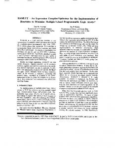
4. Algorithm In section 4.1 we solve Problem 1 and in sections 4.2 and 4.3 we solve Problem 2. 4.1. Buffer Chain for Single Sink For this problem we have a chain of buffers between the source and the sink. We define the variables of the problem to be the electrical efforts of the n buffers h1, h2, ..., hn. (cf. Fig. 1). h1

h2

hn

C1

C2

Cn

electrical effort

Lambert ( p inv ⁄ e ) λ ( p inv ) = --------------------------------------------------------------------p inv ( L ambert ( p inv ⁄ e ) + 1 )

CL

Fig. 1: Buffer Chain. Thus the overall area as a function of n and hi,s would be: n

n

∑

Ci =

i=1

∑ i=1

CL -----------n

(2)

∏ hj =

j i The goal would be to find n and all hi,s to minimize the area while both the timing and input capacitance constraints are satisfied. Theorem 1. The delay of the optimum buffer chain solution for Problem 1 is exactly equal to the specified required time TR.

Proof: For the sake of brevity we do not go through the details of the proof and just mention that the area is a monotonically decreasing function of all hi’s and since the delay along the path for some n is npinv+Σhi we can always increase some hi to decrease the area till we get to the point where the delay is equal to the required time. ■

To find the optimum number of stages n, we use the maximum input capacitance constraint C 1 ≤ C in . The input capacitance for the first buffer is computed as follows: CL C 1 = ----------∏ hi

(3)

Using equation (3), the input capacitance constraint can be restated as follows: H =

CL

∏ hi ≥ ------C

(4)

in

Theorem 2. H achieves its maximum value when all hi’s are equal. Proof: According to Theorem 1, the summation of all hi’s is constant for any given number of buffers. Since the product of some variables with a constant summation is maximum when all the variables are equal, all hi’s have to be equal to maximize H. ■

The n buffers have parasitic delay of npinv thus the overall effort delay for the whole path would be TR-npinv where TR is the required time at the sink, or the delay through the whole path according to Theorem 1. This implies that: T R – np inv hˆ i = hˆ = ------------------------n

(8)

The function Lambert(ω) is the solution to the nonlinear equation xex=ω. For further information about Lambert function refer to [2]. It is interesting to note that:

Input Cap

Area ( n ) =

Fig. 2: Plot of H = Max ( ∏ h i ) vs. n. H is drawn in Fig. 2. By taking the derivative of H and setting it equal to zero, we find that it has its maximum value at: (7) nˆ = T R × λ ( p inv ) where:

∀i = 1, …, n (5) So the maximum of H, named H as a function of n would be:

1 lim λ ( p inv ) = --e

p inv → 0

which allocates the well-known gain of e to each buffer [5]. With these observations, we propose the algorithm in Fig. 3 to find the optimum number of buffers and also the optimum sizing for them. algorithm OptN (Cin, CL, TR, P) 1. begin 2. 3. 4. 5. 6.

T R – np inv n C L  - ; ( n˜ 1, n˜ 2 ) = solve   ------------------------- = ------  n Cin n1= n˜ 1 or n˜ 1 + 1 depending on P; n2=min ( n˜ 2 , TR/Pinv);

for n=n1, ..., n2 step 2  Min  { h} =   ST 

Area ( n ) C 1 ≤ C in delay ≤ T R

7. return (best n, best {h}); 8. end; Fig. 3: Algorithm OptN. Note that for a certain n, we can have different hi,s that result in different areas and input capacitances. Among all the values that hi’s can assume, only those which result in H larger than CL/ Cin satisfy the input capacitance constraint (cf. equation (4)). In other words, only the points above the line CL/Cin are acceptable. Thus for Case I in Fig. 2 there is no feasible solution. To find the optimum solution, we intersect the line CL/Cin with the graph H (cf. line 2 of Fig. 3 and Case III in Fig. 2) which results in n˜ 1 and n˜ 2 . Note that there always exists an n˜ 1 unless the line is passing below unity and that means CL is less than Cin which has the trivial solution of “no buffers”. On the other hand there exists an upper-bound on the number of buffers because of the intrinsic delay which has to be less than the delay of the whole path, that is the number of buffers has to be less than TR/

Pinv (cf. line 3 of Fig. 3). Therefore the optimum n lies between n˜ 1 and n2. Any n smaller than n˜ 1 or larger than n2 has H below the line CL/Cin and is thus unacceptable. There is a possibility that the line CL/Cin intersects the graph but there is no integer n between the points of intersection to satisfy the polarity constraint. This only happens when the line crosses the H curve very close to the peak of the graph (cf. Case II in Fig. 2). In step 5 we find the optimum sizing for the buffers on the chain. This is the minimization of a posynomial function with posynomial inequality constraints [7] which can be easily solved in polynomial time. Finally among all the solutions, the best one in terms of the area is selected as the optimum solution. Theorem 3. The algorithm OptN solves Problem 1 optimally. Proof: Since all the feasible solutions are explicitly considered, the algorithm finds the optimum solution. ■

4.2. Buffer Tree for Multiple Sinks In this section we consider the more general case when the source Q is driving more than one sink. [4] introduced two transformations that can be performed on the fanout tree namely merging and splitting. Here we use the splitting transformation and show that splitting does not degrade the quality of the solution. h

C1 C2 h

Fig. 4: Split/Merge Transformations. Theorem 4. The split/merge operations preserve input capacitance (thus area) and delay. Proof: Suppose the gain of the original buffer is h thus the delay through the buffer for both of the branches is h+pinv and the input capacitance is (C1+C2)/h which is also the area of the buffer. After splitting the original buffer to two buffers with equal gains of h, the delay for both branches would still be h+pinv and the input capacitance would be C1/h+C2/h thus the same input capacitance and the same area. ■

Therefore if T* is the optimal fanout tree with proper sizing of buffers, it can be split to a fanout-free tree consisting of a set of buffer chains T, which has the same area as T* and also satisfies the timing and input capacitance constraints. We will find T using the optimal algorithm presented in section 4.1 and in section 4.3 we transform T to T*. The problem formulated as Problem 1 in section 2 was stated such that the maximum allowed input capacitance was given. So before we can break down the whole problem into smaller problems of optimal buffer chains, we need to somehow allocate portions of Cin to each chain (cf. Fig. 5). CL1

Cin

Cim

We introduce k new variables xk for k=1, ..., m such that:

(10) C ik = C k + x k Our heuristic is to find xk,s in such a way that their ratio is proportional to the slope of the graph in Fig. 2. The motivation behind this heuristic is the fact that between two branches, the one with smaller slope gains a larger change in the number of buffers when there is a small change in input capacitance (moving the line C Lk ⁄ C ik ). Compare this with the branch with a large slope, which would gain a smaller change in the number of buffers when there is the same change in its input capacitance. We estimate this slope with the difference of the top point and the minimal point of the graph for H. The number of stages that leads to the maximum H was computed by equation (7). With all these we propose our heuristic as in Fig. 6. algorithm InCapAlloc (Cin, {CL}, {TR}) 1. begin 2. for k=1, ..., m CL k -; C k = ---------------------------µ ( T R , p inv ) k

h

Ci2

(9)

k

4.

Split

C2

Ci1

CL k C k = ---------------------------µ ( T R , p inv )

3.

C1

Merge

the value of Hk(nk) when nk is calculated from (7), thus the minimum acceptable input capacitance would be:

CL2

CLm

Fig. 5: Input capacitance budgeting for a fanout-free buffer tree. In this section we propose a heuristic for doing this allocation. Assume m to be the number of sinks and thus the number of branches. Consider the kth branch (k=1, ..., m). The graph depicted in Fig. 2 shows that Hk, the product of buffer gains, has its minimal value of 1 at nk=0 (lim H when n tends toward 0). On the other hand, Hk cannot be any larger than µ ( T Rk, p inv ) that is

{x}=solve: m

  ∑ ( Ck + xk ) = Cin   k=1  ∀k = 2, …, m   µ (  x1  T R 1, p inv ) – 1  T R k λ ( p inv )  ----- =  ------------------------------------- ×  --------------------------  xk  µ ( T Rk, p inv ) – 1  T R 1 λ ( p inv )  5. for k=1, ..., m

6. Cik=Ck+xk; 7. return ({Ci}); 8. end Fig. 6: Algorithm InCapAlloc. After finding the allocated input capacitances, we will end up with m sub-problems that can be optimally solved by the algorithm presented in section 4.1 4.3. Merging Buffer Chains So far, we have been assuming to have a continuous-sized buffer library. In reality the ASIC library has a finite (and hopefully large) number of gate sizes. So we need to map the solution to one consistent with the library. The main problem during this transformation is that due to round-up errors, the total gate area might be significantly increased. For example a buffer size of 0.35 will be mapped to a buffer size of 1. Now, if we could merge two buffers of size 0.35 each to one buffer of size 1, the area increased is minimized. This is the main rationale for doing merging (transforming T to T* in our terminology), something similar to the split transformation but in the other way(cf. Fig. 4). Clearly we also have to be concerned about satisfying the timing constraints of using this transformation. We want to do the merging in such a way that all the timing constraints still be satisfied and the area (as well as the input capacitance of the very first stage) be the same. Very similar to the proof of Lemma 1, it can be proved for the merging transformation to have exactly the same area and delay, the electrical effort of the buffers to be merged should be the same. Since we optimize each branch with respect to the corresponding sink, the electrical efforts of buffers may not necessarily be equal. Thus we define a constant ε and merge two buffers as long as the difference between the gains of them is less than or equal to ε percent. The merging is done starting at the source of the signal, proceeding towards the sinks preserving the area while merging so as not to increase the capacitive load imposed on the previous stage beyond its expected load.

5. Experimental Results We have three different groups of experiments. In the first group, we compare the results of LEOPARD in section 4.1 with an algorithm that minimizes the delay through the path. We have implemented the algorithm presented by Sutherland to minimize the delay. The results of our algorithm are compared with the results of our implementation of Sutherland’s in Table 1. Sutherland

LEOPARD w/ 5% slack

LEOPARD

Prob#

Delay

Area

Delay

Area

Delay

Area

1 2 3 4 5 6

5.78 5.66 5.66 4.48 6.87 9.52

233 19 39 65 43 225

5.78 5.66 5.67 4.48 6.88 9.52

225 19 36 62 40 213

6.00 6.00 6.00 5.00 7.00 9.60

190 15 30 20 20 123

Table 1: Comparison with Sutherland.

For all the experiments in Table 1, the minimization problems of our algorithm were solved using Matlab Optimization Toolbox ver. 1.5.2. We first minimized the path delay with a maximum input capacitance constraint using Sutherland’s method. Then we used this minimum delay as our timing constraint for minimizing area. In the 2nd and 3rd columns, we present Sutherland’s results, and in the 4th and 5th columns we give our results for the same delay values. As expected, the area and delay results are almost the same. However when we give LEOPARD a 5% additional slack, we can reduce the area by an average of 38% as shown in columns 6 and 7. Next we show the comparison of LEOPARD results with the results of our implementation of Kung’s algorithm [4]. Kung Prob# Sinks 1 2 3 4 5 6 7 8 9 10

3 5 5 12 17 10 15 4 4 4

LEOPARD

LEOPARD +5% InCap

InCap

Area

InCap

Area

InCap

Area

46.15 51.69 53.28 160.99 432.13 426.59 101.06 54.57 110.80 27.70

176 611 916 2025 3375 2304 4230 664 571 455

46.15 51.69 53.28 160.99 432.13 426.59 101.06 54.57 110.80 27.70

175 609 913 2002 3344 2284 4183 658 566 450

48.45 54.27 55.94 169.04 453.74 447.91 106.11 57.29 116.34 29.08

154 504 739 1599 2743 1901 3333 551 479 356

Table 2: Comparison with Kung.

We used Kung’s algorithm to minimize the input capacitance and then used this minimum input capacitance as the input capacitance constraint for our area minimization problem (same input capacitance and with an additional 5%). We have assumed pinv=0.6. As can be seen in Table 2, we reduce the area by an average of 20%. Finally our last set of experimental results compare LEOPARD with fanout optimization programs of SIS. SIS runs different fanout optimization programs namely LT-Tree, Two-Level, Bottom-Up and Balanced and the best one is reported. In this experiment, we used a standard cell library consisting of ten different inverters. For each inverter we specified τintrinsic and Rout for the SIS library delay model and pinv and τ for the Sutherland delay model. We assumed that there is a perfect match between the SIS and Sutherland delay model values for each inverter. We first used the fanout optimization programs of SIS to do fanout optimization. The results are reported in column 6. Then we used the delay and input capacitance results of SIS as constraints of our problem. The results assuming continuous-size buffer library are reported in column 3. Then we performed merging and mapping to the real buffers in the discrete-size buffer library and the results are shown in columns 4 and 5. As

shown in the table, in case of continuous sizing the area is expressed in terms of the capacitances but for the discrete-sized buffers, it is the actual buffer area extracted from the library. Table 3 shows an average of 38% area improvement for LEOPARD. LEOPARD cont. sizing

LEOPARD discrete sizing

SIS

Prob#

Sinks

Σcap

Σcap

Area

Area

1 2 3 4 5 6 7

12 6 21 14 21 12 16

0.093 0.032 0.065 0.093 0.060 0.045 0.087

0.093 0.039 0.088 0.093 0.089 0.062 0.110

3920 3902 6090 3920 7220 4814 6327

5281 4676 20952 5281 11952 7857 12315

Table 3: Comparison with SIS.

6. Conclusions This paper has presented an optimal algorithm for buffer chains to minimize the area. The algorithm finds the optimum number of buffers and the optimum sizing for them by solving a posynomial minimization problems subject to posynomial inequality constraints which can be easily and quickly solved by a convex program solver. Based on this algorithm, a heuristic method was presented for the general case of buffer trees. Considering the fact that the number of discrete sizes for buffers in typical libraries has highly increased, the near-continuous buffer library is fairly accurate. The next step in improving the present work is by considering the wiring effect because the wiring effects have been proved to dominate in designs using deep sub-micron technologies. We are considering two approaches to tackle the wiring problem. The first approach is to start with the given placement of cells and routing trees and then solve the fanout optimization problem. The second approach is to try to simultaneously size and place the buffers given only the locations of the cells and not the routing structure. Each approach has its own pros and cons. The advantage to the first approach is that since we have the routing information, we actually have a better and more accurate estimation of the wire capacitance but the disadvantage is that the buffers would be restricted to be placed on the given routing tree while it could have been the case that we get a better solution if we were to do the placement and routing again. The second approach on the other hand has the advantage of performing fanout optimization and placement simultaneously but is a very hard problem because there is no accurate estimation of the wire capacitance.

7. References [1] C. Leonard Berman and J. Lawrence Carter, and K. F. Day, “The Fanout Problem: From Theory to Practice” In C. L. Seitz editor, Advanced Research in VLSI: Proceedings of the 1989 Decennial Caltech Conferences, pages 69 - 99. MIT Press, March 1989. [2] Robert M. Corless, G. H. Gonnet, D. E. G. Hare D. J. Jeffrey, and D. E. Knuth, "On the Lambert W Function", Advances in Computational Mathematics, volume 5, 1996, pp. 329-359. [3] K. Kodandapani, J. Grodstein, A. Domic and H. Touati, “A Simple Algorithm for Fanout Optimization using High-Performance Buffer Libraries”, Proceedings of ICCAD, 1993, pp. 466-471. [4] David S. Kung, “A Fast Fanout Optimization Algorithm for Near-Continuous Buffer Libraries”, Proceedings of 35th DAC, 1998, pp. 352-355. [5] C. Mead and L. Conway, “Introduction to VLSI Systems”, Addison Wesley, 1980. [6] Ivan E. Sutherland and Robert F. Sproull, “Logical Effort: Designing for Speed on the Back of an Envelope”, Advanced Research in VLSI, Univ. of Calif., Santa Cruz, 1991. [7] P. M. Vaidya, “A New Algorithm for Minimizing Convex Functions Over Convex Sets”, Proceedings of IEEE Foundations of Computer Science, Oct. 1989, pp. 332-337.