Building a Data Mining Query Optimizer - CiteSeerX

Building a Data Mining Query Optimizer Raj P. Gopalan

Tariq Nuruddin

Yudho Giri Sucahyo

School of Computing Curtin University of Technology Bentley, Western Australia 6102

{raj, nuruddin, sucahyoy} @computing.edu.au ABSTRACT In this paper, we describe our research into building an optimizer for association rule queries. We present a framework for the query processor and report on the progress of our research so far. An extended SQL syntax is used for expressing association rule queries, and query trees of operators in an extended relational algebra for their internal representation. The placement of constraints in the query tree is discussed. We have developed an efficient algorithm called CT-ITL for lower level implementation of frequent item set generation which is the most critical step of association rule mining. The performance evaluations show that our algorithm compares well with the most efficient algorithms available currently. We also discuss further steps needed to reach our goal of integrating the optimizer with database systems.

Keywords Knowledge discovery and data mining, query optimization, association rules, frequent item sets.

1. INTRODUCTION Data mining is used to automatically extract structured knowledge from large data sets. Among the different topics of research in data mining, the efficient discovery of association rules has been one of the most active. Association rules identify relationships among sets of items in a transaction database. They have a number of applications such as increasing the effectiveness of marketing, inventory control and stock location on the shop floor. Since the introduction of association rules in [1], many researchers have developed increasingly efficient algorithms for their discovery [3], [8], [11], [19]. As the computational complexity of association rules discovery is very high, most of the research effort has focused on the design of efficient algorithms. These algorithms generally use simple flat files as input and are not integrated with database systems. Imielinski and Mannila [9] identified the need to develop data mining systems similar to DBMSs that manage business applications. They also suggested developing features such as query languages and query optimizers for these systems. A number of tightly coupled integration schemes between data mining and database systems have been reported. Agrawal and Shim described the integration of data mining with IBM DBS/CS RDBMS using User Defined Function (UDF) [2]. Exploration of different architectural alternatives for database integration and comparisons between them on performance, storage overhead, parallelization, and inter-operability were presented in [17]. Recently, the impact of file structures and systems software support on mining algorithms was discussed in [16]. However,

most of these proposals focus on enhancing existing DBMSs for Data Mining and do not deal with the problem of integrating the data mining algorithms with database technology to support data mining applications. Several researchers have proposed query languages for discovering association rules. Imielinski et al. introduced the MINE operator as a query language primitive that can be embedded in a general programming language to provide an Application Programming Interface for database mining [10]. Han et al. proposed DMQL as another query language for data mining of relational databases [7]. Meo et al. described MINE RULE as an extension to SQL, including examples dealing with several variations to the association rule specifications [12]. However, all these proposals focus on language specifications rather than algorithms or techniques for optimizing the queries. Chaudhuri suggested that data mining should take advantage of the primitives for data retrieval provided by database systems [4]. However, the operators used for implementing SQL are not sufficient to support data mining applications [9]. Meo et al. gave the semantics of the MINE RULE operator using a set of nested relational algebra operators [12]. Probably because their objective was only to describe the semantics of MINE RULE, the expressions of their algebra are far too complex for internal representation of queries or for performing optimization. In this paper, we discuss our research into building a mining query optimizer that can be integrated with database systems using a common algebra for the internal representation of both data mining and database queries. We describe the general framework of the optimizer and report on our progress so far. We have focused our efforts on the critical components needed for building the optimizer. We specify an extended SQL syntax for expressing association rule queries. The queries are represented internally as query trees of an extended relational algebra. The algebraic operators are grouped into modules to simplify the query tree. Several constraints that reduce the number of association rules generated can be integrated with the different modules. Alternative execution plans may be generated, by assigning algorithms to implement various operations in the query tree, from which an optimal plan can be chosen based on cost estimates. We have developed an efficient algorithm called CT-ITL for lower level implementation of frequent item set generation which is the most critical step of association rule mining. The performance evaluations show that our algorithm compares well with the most efficient algorithms available currently. The algorithm and comparisons of its performance with other wellknown algorithms on some typical test data sets are presented. We

The Australasian Data Mining Workshop Copyright  2002

also discuss further steps needed to reach our goal of integrating the optimizer with database systems.

The main goal of this stage is to identify ways to execute the operators in the query tree.

The structure of the rest of this paper is as follows: In Section 2, we provide the framework for building an optimizer for data mining systems. In Section 3, we discuss the query language and the algebraic operators used in the query tree. The integration of constraints into the query tree is also dealt with in this Section. In Section 4, we present our algorithm for mining frequent item sets along with an evaluation of its performance and also comparison with other algorithms. Section 5 contains the conclusion and pointers for further work.

1. Accept Query

2. Translation into Algebra

3. Logical Transformation

2. DEFINITION OF TERMS AND OPTIMIZER FRAMEWORK

4. Select Algorithms to Implement Operators

In this Section, we define the terms used in describing association rules and then describe the framework of the optimizer.

5. Generate Alternative Plans

2.1 Definition of Terms We give the basic terms needed for describing association rules using the formalism of [1]. Let I={i1,i2,…,in} be a set of items, and D be a set of transactions, where a transaction T is a subset of I (T ⊆ I). Each transaction is identified by a TID. An association rule is an expression of the form X ⇒ Y, where X ⊂ I, Y ⊂ I and X ∩ Y = ∅. Note that each of X and Y is a set of one or more items and the quantities of items are not considered. X is referred to as the body of the rule and Y as the head. An example of association rule is the statement that 80% of transactions that purchase A also purchase B and 10% of all transactions contain both of them. Here, 10% is the support of the item set {A, B} and 80% is the confidence of the rule A ⇒ B. An item set is called a large item set or frequent item set if its support is greater than or equal to a support threshold specified by the user, otherwise the item set is small or not frequent. An association rule with the confidence greater than or equal to a confidence threshold is considered as a valid association rule.

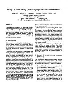
2.2 Optimizer Framework As shown in Figure 1, the optimizer framework consists of seven stages similar to the process structure of relational query optimizers. These stages are described below. Stage 1: Accept Query. The user submits a query written in a suitable query language. The query is parsed and checked for correct syntax. We use SQL extended with features of MINE RULE operator proposed by Meo et al. [12] as our query specification language. The language syntax is given in the next section. Stage 2: Translation into Algebra. The parsed user queries are translated into an extended nested algebra that will be presented in Section 3. As the extended algebra is a super set of nested algebras for expressing database queries, it is suitable for representing both database and data mining queries. Stage 3: Logical Transformation. As in traditional query optimisation, the objective of this stage is to reduce the size of intermediate results by using transformations that are independent of data values. The incorporation of mining constraints into the query tree is performed in this stage. Stage 4: Select Algorithms to Implement Operators. There are several possible low-level algorithms to implement each operator.

6. Evaluate the Cost of Alternative Plans

7. Generate an Execution Plan

Figure 1. The optimizer framework Stage 5: Generate Alternative Plans. Alternative plans are generated from combinations of alternative algorithms for the various operators. In a plan, every node of the query tree is associated with an algorithm to execute the corresponding operator. The plans can include existing data mining algorithms such as Apriori, OP, Eclat, and CT-ITL as alternative low-level procedures. Stage 6: Evaluate the Cost of Alternative Plans. Suitable formulae are to be used to compute the cost of execution of each algorithm so that the cost of alternative query plans can be estimated. The cost of a plan is estimated by considering all its operations. Stage 7: Generate an Execution Plan. The plan that has the lowest cost is chosen as the execution plan.

3. BUILDING THE QUERY TREE In this section, we describe the construction of query trees in the optimizer. First, we present the query language and the algebraic operators. It is followed by the description of a sample query tree and the grouping of operators into modules. We also discuss the integration of constraints into the query tree.

3.1 Query Language As mentioned in Section 2, we use SQL extended with the features of MINE RULE as our query specification language. We have developed a parser and a syntax checker for it (see Figure 2 for the syntax). The query is divided into two blocks: Data Preparation Block (DPB) and MINE RULE Specification Block (MSB). DPB is used to specify the preparation of input data for the mining algorithm. Its syntax is similar to that of traditional SQL queries. MSB is used to specify the parameters such as support threshold and confidence threshold for data mining applications.


For example, a query to extract association rules on items having price greater than $200 from Sales table with support threshold 20% and confidence threshold 30%, can be expressed as follows:

fall below the minimum support, minsup are pruned and the support value, sup is computed in Step 5. Table 1. Nested algebra operators

MINE RULE SimpleAssociations AS SELECT 1..n item AS BODY, 1..1 item AS HEAD, SUPPORT, CONFIDENCE WITH SUPPORT 0.2, CONFIDENCE 0.3 FROM Sales WHERE price > 200 GROUP BY tid; MINERULE SPECIFICATION BLOCK := MINE RULE AS SELECT , [, SUPPORT] [, CONFIDENCE] WITH SUPPORT , CONFIDENCE [ WHERE ] DATA PREPARATION BLOCK FROM [ WHERE ] GROUP BY [ HAVING ] [ CLUSTER BY [ HAVING ] ] := [ ] AS BODY := [ ] AS HEAD := .. ( | N) := AttributeName | {, }

No 1

Operator SELECT (σ )

2

PROJECT (π )

3

JOIN ( )

4

GROUPING (ℑ)

5

CARDINALITY (ς) NEST (Γ)

6

Figure 2. SQL extended with features of MINE RULE Selecting items with price greater than $200 is an example of a simple query constraint. With our syntax, users can include constraints in MSB and DPB (see Section 3.4).

7

UNNEST (η )

8

POWERSET (℘ )

3.2 Operators of the Algebra As indicated in [9], existing operators of SQL need to be extended for data mining applications. In this paper, we use an extended nested relational algebra for expressing data mining queries. The concepts of nested relations are an integral part of current object-relational database systems, and nested algebra operations are integrated into most of the object-relational query languages. The operators needed for expressing association rule queries are shown in Table 1, where each operator is described briefly.

Description Returns a collection of tuples in a relation that satisfy a given condition. The condition can include set comparisons. Returns existing attribute values or new attribute values computed by functions specified as Lambda expressions. It can also be used to rename attributes. Combines every pair of related tuples of two specified relations that satisfy the join condition into a single tuples of the result relation. Join condition can include set comparisons. Groups tuples based on the grouping attributes and computes aggregate functions (average, count, max, min, sum, etc.) on other specified attributes. Counts the number of values of a set valued attribute in each tuple of a relation. Groups tuples together based on common values of specified nesting attributes. The resulting relation will contain exactly one tuple for each combination of values of the nesting attributes. Undoes the effect of NEST, restructures the set of tuples and flattens out the relation so that each set member (tuple) may be examined individually. Generates a powerset of values in a specified attribute. For a specified set valued attribute containing n values in a tuple, the POWERSET operator generates a tuple in the output relation, by replacing the input set value by its n 2 −1 subsets (∅ is not included ).

3.3 Query Tree for Association Rules Mining The query tree in Figure 3 represents the example of association rules query given in Section 3.1. Grouping of operator sequences into modules simplifies the query tree as shown in Figure 3a. These modules correspond to the commonly recognized steps in association rule mining: data preparation, frequent item set mining, and association rule generation. In Step 1 of Figure 3b, the attributes tid and item are projected from the input relation R, and the tuples are nested on tid in Step 2. In Step 1 of Figure 3c, the powerset of items for each tid is generated. The output of this step is unnested on the item set attribute in Step 2 so that the number of occurrences of each item set can be counted in Step 3. In Step 4, the item sets that would

In Step 1 of Figure 3d, two copies of large item sets (A and B) are used as input. They are joined on the condition that the item set of a tuple in A is a proper subset of the item set of a tuple in B. In Step 2, the attributes are renamed to identify the smaller item set as body (BD) of potential rules and its corresponding larger item set as superset (sp). In step 3, the confidence values for candidate association rules are computed and then rules that have confidence greater than or equal to the confidence threshold are selected in Step 4. In Step 5, the head (HD) of the rules are obtained by applying the set difference operator, and the result consisting of the body (BD), head (HD), support and confidence are projected for all valid


rules. More examples of query trees representing typical association rule queries can be found in [5]. Generate Association Rules Generate Frequent Item Sets

Data Preparation

σ price > 200 Sales

(a) Basic Query Tree Γ(tid)

(2)

(1) π(λr 〈(tid, r.tid), (item, r.item)〉) (b) Data Preparation (5)

efficient implementation. All the existing algorithms for frequent item set mining can be viewed as computing a partial power set of item sets present in the transactions. Instead of generating all the item sets first and then testing for support as in the query tree of Figure 3c, they try to limit the generation of item sets to those satisfying the minimum support constraint. These algorithms adopt strategies to test the support of item sets as they are generated as well as to avoid generating item sets that cannot possibly have minimum support. We have also developed an efficient algorithm that can replace the frequent item set module of the query tree in actual implementation. This algorithm will be discussed in Section 4.

3.4 Integrating Constraints into the Query Tree Specification of constraints in mining queries can reduce the volume of uninteresting rules generated, as well as allow greater focus on the user’s needs and interests at the application level. The importance of constraint-based mining has been highlighted by recent work in this area [13], [14]. A significant advantage of the algebraic query tree representation is the insight it provides for dealing with constraints in mining queries. A categorization of constraints at the application level was proposed in [13] as follows: 1.

Item Constraint: Specifies what are the particular individual or groups of items that should or should not be present in the pattern. E.g., mine only beverage products.

2.

Length Constraint: Specifies restrictions on the length of patterns. E.g., mine only transactions with at least five items.

3.

Model-based Constraint: Looks for patterns that are sub- or super patterns of some given patterns (models). For example, a shop manager may be interested in what other goods a customer is likely to buy if she buys ‘Pepsi’ and ‘Hot Dog’.

4.

Aggregate Constraint: For items in a pattern, find aggregates such as MAX, MIN, AVG, and SUM. For example, a shop manager wants to find frequent item sets where the average price of items is $50.

π(λr 〈(freq_itemset, r.itemset), (sup, r.count_tid /n)〉)

(4)

σ count_tid ≥ n ∗ minsup

(3)

itemsetℑcount tid

(2)

η (itemset)

(1) π(λr 〈(tid,r.tid), (itemset,℘(r.item))〉) (c) Generate Frequent Item Sets (5)

(4)

π (λr 〈(BD, r. BD), (HD, r.sp− r.BD ), (sup, r.sp_sup), (conf, r.conf)〉)

σ conf

≥

minconf

The main idea for efficient processing of constrained queries is to push the constraints down the query tree, so that the size of intermediate results is reduced. The types of constraints that can be processed in each module of the query tree are discussed below. 1.

(3) π(λr 〈(BD, r.BD), (BD_sup, r.BD_sup), (sp,r.sp), (sp_sup, r.sp_sup), (conf,(r.sp_sup/r.BD_sup)〉) (2) π (λr 〈(BD, r.A.freq_itemset), (BD_sup, r.A.sup), (sp, r.B.freq_itemset), (sp_sup, r.B.sup)〉) (1)

A.freq_itemset ⊂ B.freq_itemset

(d) Generate Association Rules Figure 3. Query Tree for Association Rules Mining A limitation of our algebra is the lack of recursion. Therefore, we have used the power set operator, although it is not suitable for


Data Preparation: Most of the current algorithms for mining association rules just use a single flat file containing a list of transactions with items. In a real application, the data input for mining could be made up from several tables requiring join, grouping, select, project and other SQL operators. Types of constraints that can be applied in this module are as follows: • • •

Item Constraint: Can be expressed as predicate of select operation. E.g., mine only beverages products. Aggregate Constraint: Constraints using aggregate functions MIN or MAX on attributes of items. E.g., mine only items with a MIN/MAX price of $100. Length Constraint: Transactions with number of items less than a given value can be filtered out. E.g., to mine all frequent item sets with length at least x, all

2.

transactions with number of items less than x can be deleted. However, this constraint will need to be applied again in the next step. • Model-based Constraint: For mining frequent item sets that contain certain items. E.g., frequent item sets with ‘Pepsi’ and ‘Hot Dog’ . In this case, all transactions that do not contain ‘Pepsi’ and ‘Hot Dog’ can be deleted. Generate Frequent Item Sets: In the query tree, all item sets are generated before they are checked for minimum support. Although actual implementation will be different as explained earlier, the processing of constraints in this module provides the basis for placing the constraints in real algorithms. Constraints that can be applied in this module are as follows:

Transaction identifiers can be ignored provided the items of each transaction are linked together.

Tid 1 2 3 4 5

Aggregate Constraint: Constraints using aggregate function AVG can only be applied in this step. Prune item sets that fail the constraint. • Length Constraint: Prune all item sets of less than x number of items. • Model-based Constraint: Prune item sets that do not contain certain items. E.g., to mine only frequent item sets with ‘Pepsi’ and ‘Hot Dog’ , remove all item sets that do not contain these. • Support Constraint: Any item set with support less than support threshold will not be included in frequent item sets. Generate Association Rules: Constraints that cannot be applied earlier are processed in this module. • • •

2 3 2 4 4

Items 3 5 7 9 4 5 12 4 5 6 11 5 8 5 10

(a) Sample Database

•

3.

1 2 1 3 3

Level 0

0 0 1

Level 1

0 0 12 1 0 2 2

Level 2 0 0 123 1 0 23 2 0 3

1

0 0 124 4 1 0 24

3

Level 3 0 1 2 3

Confidence Constraint: Any rule with confidence less than confidence threshold will not included in the output. Item Constraint: User may require specific items in the left hand side (LHS) or specific items in the right hand side (RHS) of the rules. Length Constraint: User may require a specified number of items in the LHS or in the RHS.

0 1 2 3 4

0 1 2 0 0

0 0 0 0

1234 4 234 34 4

0 1 1235 5 1 0 235 2 0 35

12345 5 2345 345 45 5

5 0 1 1245 1 0 245

Level 4

(b) Compressed Transaction Tree ITEMTABLE Index 1 2 3 4 5 Item 1 2 3 4 5 Count 2 3 4 4 5

4. ALGORITHM FOR GENERATING FREQUENT ITEM SETS

TRANSLINK

We focus on mining frequent item sets since it is computationally the most expensive module. In this section, we describe our most recent low-level algorithm for generating frequent item sets. A performance comparison of our algorithm with other similar algorithms is also presented.

t1

2 3 4 5

Count 1 1 2 2

t2

1 2 3 5

1 1

t3

1 2 4 5

1 1

4.1 Transaction Tree and ITL Data Structure Researchers have proposed various data representation schemes for association rules mining. They can be classified as horizontal, vertical, or a combination of the two. Algorithms like Apriori and its variants use horizontal data layout, Eclat uses vertical data layout, and algorithms like FP-Growth and its extensions use a combination of vertical and horizontal data layouts. The optimizer will choose the best algorithm based on the dataset characteristics and other important factors (index availability etc.). We have developed a generic data structure Item-Trans Link (ITL) that can be used for most algorithms. The data representation in ITL is based on the following observations: 1) Item identifiers may be mapped to a range of integers; 2)

(c) ITL Figure 4. Compressed Transaction Tree and ITL Data Structure ITL consists of an item table (named ItemTable) and the transactions linked to it (TransLink). ItemTable contains all individually frequent items where each item is stored with its support count and a link to the first occurrence of that item in TransLink. TransLink represents each transaction of the database that contains items of ItemTable. The items of a transaction are


Each node of the tree will contain a 1-freq item and a set of counts indicating the number of transactions that contain subsets of items in the path from the root as shown in Figure 4c.

arranged in sorted order and for each item, there is a link to the next occurrence of that item in another transaction.

For example, using the sample database shown in Figure 4a, and minimum support of 2 transactions, we create a compressed transaction tree of 1-frequent items as in Figure 4b, before mapping it to ITL in Figure 4c. Each node in the compressed transaction tree has additional entries to keep the count of transactions represented by the node. For example, the entry (0,0) at the leaf node of the leftmost branch of the tree represents the item set 12345 that incidentally does not occur in the sample database. The first 0 in the entry indicates that the item set starts at level 0 in the tree which makes 1 the first item. The second 0 indicates that no transaction in the database has this item set. Similarly, the entry (1,1) means there is one transaction with item set 2345 and (2,2) means there are two transactions with item set 345. In the implementation of the tree, the counts at each node are stored in an array so that the level for an entry is the array index that is not stored explicitly. The doted rectangles in Figure 4b, that show the item sets corresponding to the nodes in the compressed tree are not part of the data structure.

3.

Construct compressed ITL: The compressed transaction tree is traversed to construct the ItemTable and TransLink.

4.

Mine Frequent Item Sets: All the frequent item sets of two or more items are mined by a recursive function following the pattern growth approach and using tid-count-intersection method.

A detailed description of CT-ITL is available in [18].

4.3 Performance Study We have compared the performance of CT-ITL with other wellknown algorithms including Apriori, Eclat [19] and OP [11]. Apriori version 4.03 is generally acknowledged as the fastest Apriori implementation available. In this new version, it uses a prefix tree to store the transactions and the frequent item sets. Eclat uses the tid-intersection in its mining process. Implementations of Eclat and Apriori were downloaded from [20]. OP is currently the fastest available pattern growth algorithm. 1000 Runtime (seconds)

We reduce the number of transactions that has to be traversed during mining, by replacing, a set of transactions containing identical item sets by a single transaction and a count. We found that this can be done efficiently using a modified prefix tree to identify transaction sets. We also developed a scheme to compress the prefix tree by storing information of identical subtrees together.

When the compressed transaction tree is mapped to ITL, information is added to each row of TransLink, indicating the count of transactions that have different subsets of items. Each node in the tree that has transaction count greater than zero is mapped to a row in TransLink, and the nonzero entries at the tree node attached to the corresponding row.

Connect-4 100

10

1 75

4.2 CT-ITL

2.

Construct the compressed transaction tree: Using the output of Step 1, only 1-freq items are read from the transaction database. They are mapped to the new item identifiers and the transactions inserted into the compressed transaction tree.

90

95

Runtime (seconds)

1000

There are four steps in CT-ITL algorithm as follows: Identify the 1-frequent item sets and initialise the ItemTable: The transaction database is scanned to identify all 1-freq items, which are then recorded in ItemTable. To support the compression scheme used in the second step, all entries in the ItemTable are sorted in ascending order of their frequency and the items are mapped to new identifiers that are ascending sequence of integers. (In Figure 4c, the change of identifiers is not reflected due to our choice of sample data.)

85

Support Threshold (%)

We have developed several algorithms for mining frequent item sets based on ITL [6], [18]. CT-ITL is the most efficient of these algorithms. The number of transactions to be traversed during mining is reduced by grouping transactions as discussed above. The number of item traversals within transactions is minimized by using tid-count intersection. Because of transaction grouping, a tid represents a group of transactions rather than a single transaction. Therefore, tid-count lists are shorter than simple tid lists, and the intersections are performed faster. 1.

80

Pumsb* 100

10

1 30

40

50

60

70

Support Threshold (%)

Apriori

OP

CT-ITL

Eclat

Figure 5. Performance comparisons of CT-ITL, Apriori, Eclat and OP on Connect-4 and Pumsb* The results of our experiments are shown in Figure 5. All programs are written in Microsoft Visual C++ 6.0. All the testing was performed on an 866MHz Pentium III PC, 512 MB RAM, 30 GB HD running Microsoft Windows 2000. In this paper, the runtime includes both CPU time and I/O time.


Several datasets were used to test the performance including Mushroom, Chess, Connect-4, Pumsb* and BMS-Web-View1. We present the result of testing on Connect-4 (67,557 transactions, 129 items, 43 is the average transactions size) and Pumsb* (49,046 transactions, 2,087 items, 50 is the average transactions size), both being dense data sets that produce long patterns even at high support levels. Connect-4 was downloaded from Irvine Machine Learning Database Repository [21]. Pumsb* contains census data from PUMS (Public Use Microdata Samples). Each transaction in it represents the answers to a census questionnaire, including the age, tax-filing status, marital status, income, sex, veteran status, and location of residence of the respondent. In Pumsb* all items of 80% or more support in the original PUMS data set have been deleted. This dataset was downloaded from [22]. Performance comparisons of CT-ITL, Apriori, Eclat and OP on these datasets are shown in Figure 5. Note that we have used logarithmic scale along the y-axis. CT-ITL outperforms all other algorithms on Connect-4 (support 80-95) and Pumsb* (support 50-70). It always performs better than other algorithms at higher support levels. As the support threshold gets lower and number of frequent item sets generated is significantly larger, the relative performance of OP improves. A detailed discussion of the results on these and other data sets can be found in [18].

4.4 Comparison with Other Algorithms We compare CT-ITL with a few well-known algorithms for frequent item set mining. In the following, we highlight the significant differences between our algorithm and others: Apriori. The Apriori algorithm combines the candidate generation and test approach with the anti-monotone or Apriori property that every subset of a frequent item set must also be a frequent item set [1]. A set of candidate item sets of length n + 1 is generated from item sets of length n and then each candidate item set is checked to see if it is frequent. Apriori suffers from poor performance since it has to traverse the database many times to test the support of candidate item sets. CT-ITL follows the pattern growth approach where support is counted while extending the frequent patterns, using a compact representation of the transaction database. As mentioned earlier, CT-ITL consistently performs better than Apriori. FP-Growth. FP-Growth algorithm builds an FP-Tree based on the prefix tree concept and uses it during the whole mining process [8]. We have used the prefix tree for grouping transactions, by compressing it significantly as described in Section 4.1. We map the tree to the ITL data structure in order to reduce the cost of traversals in the mining step using tidintersection. The cost of mapping the tree to ITL is justified by the performance gain obtained in the mining process. FP-Growth uses item frequency descending order in building the FP-Tree. For most data sets, descending order usually creates fewer nodes compared to ascending order. In CT-ITL, a tree with fewer nodes but more paths will run slower compared to a tree with more nodes but fewer paths. From our experiments, it was found that CT-ITL is faster using ascending order than with descending order although the number of nodes is usually fewer with descending order. Eclat. Tid-intersection used by Zaki in [19] creates a tid-list of all transactions in which an item occurs. In our algorithm, each tid in

the tid-list represents a group of transactions and we need to note the count of each group. The tid and count are used together in tid-count intersection. The tid-count lists are shorter because of transaction grouping and therefore perform faster intersections. H-Mine. In the mining of frequent item sets after constructing the ITL, our algorithm may appear similar to H-Mine [15] but there are significant differences between the two as given below. In the ITL data structure of CT-ITL, each row is a group of transactions while in H-struct, each row represents a single transaction in the database. Grouping the transactions significantly reduces the number of rows in ITL compared to Hstruct. After the ITL data structure is constructed, it remains unchanged while mining all of the frequent patterns. In H-Mine, the pointers in the H-struct need to be continually re-adjusted during the extraction of frequent patterns and so needs additional computation. CT-ITL uses a simple temporary table called TempList during the recursive extraction of frequent patterns. CT-ITL need to store in the TempList only the information for the current recursive call which will be deleted from the memory if the recursive call backtracks to the upper level. H-Mine builds a series of header tables linked to the H-struct and it needs to change pointers to create or re-arrange queues for each recursive call. The additional memory space and the computation required by H-mine to extract the frequent item sets from H-struct are significantly more than for CT-ITL. OpportuneProject (OP). OP is currently the fastest available program based on pattern growth approach. OP is an adaptive algorithm that can choose between an array or a tree to represent the transactions in the memory. It can also use different methods of projecting the database while generating the frequent item sets. However, OP is essentially a combination of FP-Growth and HMine. H-Mine does not compress the transactions as in our algorithm and the FP-Tree is significantly larger than our compressed transaction tree. As discussed in Section 4, our compression method makes CT-ITL perform better than OP on several typical datasets and support levels.

5. CONCLUSION In this paper, we have reported on our progress in building the components of a data mining query optimizer. A framework for the optimizer was presented in Section 2. It consists of seven stages. The research has progressed to Stage 4 of this framework, with our efforts focused on constructing the critical components. We have developed a parser and syntax checker for the query language, as well as an extended algebra and query tree for internal representation of mining queries. Constraints are integrated into the query tree, as briefly discussed in Section 3. Further, we have developed an efficient algorithm for implementing the most critical module of the query tree. Work is in progress to integrate the processing of constraints into this algorithm. Further work is needed to generate alternative plans by assigning algorithms to all the modules of the query tree. We also have to develop cost models for estimating the cost of different algorithms and of potential query plans.


6. ACKNOWLEDGMENTS We are thankful to Junqiang Liu for providing us the OpportuneProject program and to Christian Borgelt for the Apriori and Eclat programs.

7. REFERENCES [1] Agrawal, R., Imielinski, T. and Swami, A., Mining Association Rules between Sets of Items in Large Databases. In Proceedings of ACM SIGMOD, (Washington DC, 1993), ACM Press, 207-216. [2] Agrawal, R. and Shim, K., Developing Tightly-Coupled Data Mining Applications on a Relational Database System. In Proceedings of the 2nd Int. Conf. on Knowledge Discovery in Databases and Data Mining, (Portland, Oregon, 1996). [3] Agrawal, R. and Srikant, R., Fast Algorithms for Mining Association Rules. In Proceedings of the 20th International Conference on Very Large Data Bases, (Santiago, Chile, 1994), 487-499. [4] Chaudhuri, S. Data Mining and Database Systems: Where is the intersection? IEEE Data Engineering Bulletin, 1998. [5] Gopalan, R.P., Nuruddin, T. and Sucahyo, Y.G., Algebraic Specification of Association Rules Queries. In Proceedings of Fourth SPIE Data Mining Conference, (Orlando, FL, USA, 2002). [6] Gopalan, R.P. and Sucahyo, Y.G., TreeITL-Mine: Mining Frequent Itemsets Using Pattern Growth, Tid Intersection and Prefix Tree. In Proceedings of 15th Australian Joint Conference on Artificial Intelligence, (Canberra, Australia., 2002). [7] Han, J., Fu, Y., Wang, W., Koperski, K. and Zaiane, O., DMQL: A Data Mining Query Language for Relational Databases. In Proceedings of SIGMOD DMKD workshop, (Montreal, Canada, 1996). [8] Han, J., Pei, J. and Yin, Y., Mining Frequent Patterns without Candidate Generation. In Proceedings of ACM SIGMOD, (Dallas, TX, 2000). [9] Imielinski, T. and Mannila, H. A Database Perspective on Knowledge Discovery Communications of the ACM, 1996, 58-64. [10] Imielinski, T., Virmani, A. and Abdulghani, A., DataMine: Application Programming Interface and Query Language for Database Mining. In Proceedings of the 2nd Int. Conf.on Knowledge Discovery and Data Mining, (1996). [11] Liu, J., Pan, Y., Wang, K. and Han, J., Mining Frequent Item Sets by Opportunistic Projection. In Proceedings of ACM SIGKDD, (Edmonton, Alberta, Canada, 2002). [12] Meo, R., Psaila, G. and Ceri, S. An Extension to SQL for Mining Association Rules. Data Mining and Knowledge Discovery, 2 (2). 195-224.

[13] Pei, J. and Han, J. Constrained Frequent Pattern Mining: A Pattern-Growth View. ACM SIGKDD Explorations, 4 (1). [14] Pei, J., Han, J. and Lakshmanan, L.V.S., Mining Frequent Itemsets with Convertible Constraints. In Proceedings of 17th International Conference on Data Engineering, (Heidelberg, Germany, 2001). [15] Pei, J., Han, J., Lu, H., Nishio, S., Tang, S. and Yang, D., HMine: Hyper-Structure Mining of Frequent Patterns in Large Databases. In Proceedings of IEEE ICDM, (San Jose, California, 2001). [16] Ramesh, G., Maniatty, W.A. and Zaki, M.J., Indexing and Data Access Methods for Database Mining. In ACM SIGMOD Workshop on Research Issues in Data Mining and Knowledge Discovery, (2002). [17] Sarawagi, S., Thomas, S. and Agrawal, R., Integrating Association Rule Mining with Relational Database Systems: Alternatives and Implications. In Proceedings of ACM SIGMOD, (1998). [18] Sucahyo, Y.G. and Gopalan, R.P. CT-ITL: Efficient Frequent Item Set Mining Using a Compressed Prefix Tree with Pattern Growth. To appear in Proceedings of 14th Australasian Database Conference, (Adelaide, 2003). [19] Zaki, M.J. Scalable Algorithms for Association Mining. IEEE Transactions on Knowledge and Data Engineering, 12 (3). 372-390. [20] http://fuzzy.cs.uni-magdeburg.de/~borgelt [21] http://www.ics.uci.edu/~mlearn/MLRepository.html [22] http://augustus.csscr. washington.edu/census/

About the authors: Raj P. Gopalan completed a MSc in Computer Science at the National University of Singapore and a PhD in Computer Science at the University of Western Australia. He is currently a lecturer in the School of Computing at Curtin University of Technology. His research interests include, Data Mining, Data Warehousing and OLAP, and Multi-media databases. Tariq Nuruddin completed a MSc in Mathematics and Statistics at the Louisiana Tech University. He is currently a graduate student at the School of Computing, Curtin University of Technology. His research interests include data mining, algebraic methods, and category theory. Yudho Giri Sucahyo completed a MSc at the Faculty of Computer Science, University of Indonesia and is currently a PhD candidate at the School of Computing, Curtin University of Technology. He is supported by an AusAID scholarship. He is also a lecturer in the Faculty of Computer Science, University of Indonesia. His research interests include, Data Mining, Database Systems and Software Engineering.
