acceleration data over a menstrual cycle, i.e., circa 30 days, and .... deplete the batteries fully before encountering brown-outs. For .... approximately once an hour. ... We observed that these missed connections occur mostly while ... We realized after the experiment was finished that our two ..... After the corrupted data are.
1
Lessons from the Hogthrob Deployments Marcus Chang, Cécile Cornou, Klaus S. Madsen, Philippe Bonnet University of Copenhagen Abstract—Today, even small-scale sensor networks need to be carefully designed, programmed and deployed to meet user goals, such as lifetime or quality of the collected data. Only by confronting the problems that do come up during actual deployments can we devise the tools, methods and abstractions that will help meet the requirements of a sensor network infrastructure. In this paper we report on the lessons we learnt deploying two experimental sensor network in a pig farm in the context of the Hogthrob project. We describe the design of the sensor networks whose goal was to collect time series of sow acceleration data over a menstrual cycle, i.e., circa 30 days, and we discuss the lessons we learnt.
remain unattended in order to avoid disturbing the sows. This is a tough challenge in terms of energy consumption as packaging constraints the size of the batteries and thus the energy budget. We deployed our sensor network in a production herd in Sjælland, Denmark2. Because of cost considerations (we need to refund the farmer for the missed opportunity to perform artificial insemination) we reserved a limited number of sows.
Index Terms—sensor network deployments, group housed sows, acceleration timeseries.
I.INTRODUCTION
I
n the context of the Hogthrob project 1, we aim at developing an infrastructure for online monitoring of sows in production (detect oestrus, detect injury, ...). Today, farmers use RFID based solutions to regulate food intake. Such systems do not allow the farmers to locate a sow in a large pen, or to monitor the life cycle of a sow (detect oestrus, detect injury, ...). Our long term goal is to design a sensor network that overcomes these limitations and meets the constraints of the pig industry in terms of price, energy consumption and availability. In a first phase, we focus on oestrus detection. We use a sensor network to collect the data that scientits can use to develop an oestrus detection model based on the sow's activity. Such sensor networks promise to be part of the experimental apparatus scientists can use to densely sample phenomena that were previously hard or impossible to observe in-situ, and then build appropriate models. Automated oestrus detection has been mainly studied for dairy cattle and for individually housed sows. Group housing complicates the problem significantly as it may impair the oestrus behaviour of subordinate sows. Possible methods for automated oestrus detection for group housed sows are reviewed in [CC06]. Our goals are (i) to assess whether it is feasible to detect the onset of oestrus using acceleration data and (ii) to devise a detection method that is appropriate for online monitoring. We designed a sensor network that collects sow acceleration data during a complete oestrus cycle (21 days in which the sows show one oestrus). In this period, the nodes should
Figure 1: Plan of the Experimental Pen We ran a first experiment during a four weeks period in February and March 2005 and a second in January and February 2007. In this paper, we report our experience preparing, conducting and analyzing these field experiments: 1. We describe the design of the sensor network. Our first experiment focused on the power budget and on energy consumption in order to keep data collection running for 3 weeks. We relied on the lessons learned from previous deployments as they were related in the literature when planning the experiment [SITEX02][GDI02][GDI04]. We thus paid particular attention to packaging, battery selection, duty cycling, and replication in the back-end infrastructure. In our second experiment, we focused on improving the yield of the experiment with a goal of 90% of accurate data collected. 2. We discuss the lessons learnt and how our results can be applied in a larger context. II.FIRST EXPERIMENT Our goal was to design a sensor network for the collection of sow acceleration data sets. We faced two key problems, typical of sensor networks deployed for scientific data collection: 1) What is our power budget? How to duty cycle the sensor nodes to keep energy consumption within our budget? 2) How to collect the data from the sensor nodes to the backend infrastructure.
1 A collaboration between DIKU, DTU, KVL, IO Technologies and NCPP (http://www.hogthrob.dk).
www.askelygaard.dk
2
2 A. Sensor Network We decided to use BTnodes [Beutel] as a hardware platform. We used Btnodes rev2, equipped with an ATMega128 micro-controller, 64 KiB of external RAM, and an Ericsson ROK 101 007 Bluetooth module. Our goal was to use the high-bandwidth radio of the BTnodes to transmit large amounts of data (434 kbit/s compared to contemporary radios like the CC1000 which only had 76.8 kbit/s bandwidth) . This opens up for a model where the sensor data is stored locally on the node as it is captured, and periodically transmitted in large chunks to the base station. Our goal is thus to leverage the radio bandwidth to reduce its duty cycle. We developed an accelerometer board for the BTnode and designed a node packaging that could fit the neck of a sow Sensor Data. In his experiment with individually housed sows, Geers [Geers95] used a sampling rate of 255 Hz. An experiment with the MIT LiveNet system used a 50Hz sampling rate to detect shivering [Sung04]. We estimated that a 4 Hz sampling rate would be good enough to capture the activity of sows. Accelerometerstoress. The most important parameter of the accelerometer, is the range of acceleration it can measure. The acceleration experienced when a human walks is in the range of 0-2g. We assume that the acceleration of a sow walking will be in the same range, while the occasional fights could lead to higher accelerations. For the sake of redundancy and comparison, we equipped our board with a 2D analog accelerometer (ADXL320 from Analog Devices) as well as a 3D digital accelerometer (LIS3L02DS from STMicroelectronics).
Packaging. We need an appropriate packaging in order to attach a BTnode to the neck of a sow. We had to design a protective casing that (a) could contain a BTnode with the accelerometer board and batteries, (b) would fit the shape of a sow’s neck and (c) would be robust enough to resist the hostile environment. We designed a box in a carved oblong form that fits the shape of a sow's neck. The box is in effect air tight (23 screws to fix the top, with an o-ring underneath, to seal it). It is 135x33x80mm. Its walls are 5 mm thick to resist bites. The box can contain a BTnode equipped with the accelerometer board as well as a pack of 4 AA size batteries. Note that the protective casing turned out to be the most expensive part of the equipment. Attaching this box to the neck of a sow was also a challenge. We finally devised a reliable method using medical tape and a sow collar. Power Budget. In our experience, BTnodes exhibit unstable behavior with an input voltage of around 3V. We thus decided to use a 4x1.2V battery pack to make sure that the node could deplete the batteries fully before encountering brown-outs. For economic reasons, we decided to use rechargeable batteries. We decided against Lithium cells because of their sensitivity to shocks and their price. We opted for NiMH batteries. We experimented with three different cells. One from Panasonic with a nominal capacity of 2100 mAh, and two Ansmann models with nominal capacities of 2300 and 2400 mAh. A constant discharge experiment confirmed the capacity figures given by the manufacturers as well as the promised flat discharge curves. Our power budget thus amounts to around 10000mWh. Duty Cycling Model This limited power budget led us to define an aggressive duty cycling model. First, we should keep
the power consumption of the BTnode in sleep mode to a minimum. Our initial experiments showed a consumption of 54 mW for an idle BTnode. We succeeded in bringing this figure down to 2,4 mW using a more aggressive sleep mode and disabling the external memory. Second, in order to duty-cycle the Bluetooth module, we have to store the data we sample from the accelerometers. This is a bit of a challenge with the external memory disabled. We decided to use the unused parts of the program memory, i.e., 128 KiB flash, inside the ATMega128 micro-controller. Among those, 8 KiB are reserved for the boot loader. Assuming our data occupies around 20 KiB, we can use around 100 KiB of program memory to store sensor data. That corresponds to around 55 minutes of sampling. We thus adopted a duty cycling model where the radio is turned off until memory is almost filled up.
Figure 2: The sensor node box. Back-end Infrastructure. For our experiment, the role of the back-end infrastructure is twofolds. First, it shoud obtain and store data from the sensor nodes. Second, it should collect ground truth about sow activity, i.e., video recording of the pen. We consider a star topology for data collections. Indeed, sensor nodes are attached to sows located in an indoors pen (approximately 200 m2), where they are all in communication range of a base station. The base station is a Bluetooth access point whose role is (a) to communicate with the sensor nodes, and (b) to timestamp and store the received packets. The communication between the sensor nodes and the base station relies on the following protocol. The base station continually sends inquiries. Whenever required by the duty cycling model, a sensor node starts an inquiry scan (a scan requires less energy than sending inquiries [Leopold03]). When a base station detects a sensor node, it creates a connection. When the connection is established, the sensor node sends some status information including the number of samples it stores. The server does the bookkeeping, it requests the samples that have not yet been transmitted and acknowledges their reception. The sensor node stores a sample until its transmission has been acknowledged. When memory is full, samples are simply dropped.
Our base station is a PC connected to an external Bluetooth dongle hanging from the ceiling in the middle of the pen. In order to check if the range of a single Bluetooth dongle provided sufficient coverage, we placed a BTnode (with its protective casing) in different corners of the pen and verified that connections could be opened and data transferred. This test did not reveal any problems. The key issues in the design of the infrastructure were the following • Timestamping: In order to analyze the data sets, we need to
3 control that a sow is actually moving when the data set indicates some activity. The time stamps of the time series must match with the time stamps from the video frames. The same PC is used to timestamp both video frames and sensor data. The PC is connected to the Internet and synchronized with a remote NTP server. The timestamping of video frames is straightforward: the frame grabbing software obtains a time stamp for each frame it captures. The timestamping of timeseries is a bit more complex.
First, each sensor node attaches a logical timestamp (a counter) to the samples it collects. Second, the PC attaches the current timestamp to each batch of samples it gets from a sensor node (in the context of one Bluetooth connection). Timestamps are attached to individual samples in a post processing phase. • Data storage: Each frame stored in PNG format occupies 8 KiB. We can thus expect a stream of 32 KiB per second for each camera and a total of 80 GiB of data per camera for the duration of the experiment. We used an ADSL line with an uplink capacity of 512 KiB/sec to connect the base station PC to the Internet. We reserved 1TB of disk space on a file server to store the video and the time series. • Reliability: We paid particular attention to reliability as it had been reported to be a problem in previous deployments [GDI02]. We chose a straightforward approach and basically replicated all the processing on two base station PCs. Both PCs were equipped with their own Bluetooth dongle. We splitted the coaxial cables so that each PC was connected to all the cameras. Both PCs ran NTP clients connected to the same NTP server. They proceeded in parallel with the timestamping of both video frames and time series. Both PCs shared the ADSL line connecting the farm to the Internet. A fail-over service monitored both servers and picked one of the PCs to upload data to the remote file server. • Resilience to the hostile environment: Sows are aggressive animals and they would try to eat any equipment they can put their mouth on. The pen is an hostile environment mainly due to the corrosive. We thus decided to place the PCs in a container outside the pen. We used USB extenders, connected via Ethernet cables, to connect the PCs to the Bluetooth dongles.
B.Field Experiment The experiment took place at Askelygaard farm from February 21st to March 21st 2005. Data was collected from the sensor network from Day 11 to Day 30. In this Section we report on the data collection process using our sensor network and we describe the collected data.
1) Hits and Misses Sensor node lifetime was our main concern when designing the sensor network. Our lab experiment suggested a possible lifetime of around 60 days. In fact, 4 of the nodes could collect data for the duration of the experiment. The fifth sensor node lost its Bluetooth module a week before the end of the experiment and was replaced. We collected battery drain information during the experiment. The battery drain was measured by the BTnode and sent to the base station in the status packet that prefixed all transmissions. Figure 3 shows the voltage drain for one of the sensor nodes equipped with an Ansmann battery pack. We obtain a flat discharge curve very
similar to the one we obtained with constant discharge. Note that the actual voltage of the cell is higher than the nominal 1.2V and we obtain around 5V for the duration of the experiment. From day 37 on, there is still enough power left in the batteries to turn the Bluetooth module on, receive a connection and send the initial packet. However during the send phase, the voltage of the batteries drops so low that the node browns out. The main problem we encountered during the experiment was missed connections between the base station and sensor nodes. We expected the sensor nodes to upload their data approximately once an hour. However, we observed an average of only 16 connections per day. Note that once a connection was established, data transfer was successful. We observed that these missed connections occur mostly while sows are in a corner of the pen. It is most probably the water contained in the body of the sow and the iron contained in the internal alcoves of the pen that limit the communication range of the sensor node. As a result our time series contain numerous holes (see next Section).
Figure 3: Voltage drain during the experiment for a sensor node equipped with an Ansmann battery pack.
Another problem was that sensor nodes rebooted every other day. The only node that did not reboot was equipped with a custom made battery pack with batteries welded together. Reboot caused the logical time stamp counter to reinitialize. As a result, the samples that had been collected but not transferred were overwritten. Fortunately, we had programmed the nodes to connect to the base station only 10 minutes after a reboot so we avoided cascading effects. We realized after the experiment was finished that our two PCs (connected to the same NTP server) were approximately 20 seconds out of sync. This problem combined with the numerous node reboots made the post-processing of the sensor data complicated and error prone. 2)Collected Data We collected around 200MiB of sensor data per node3. We validated a posteriori the validaty of the data collected from the analog and digital accelerometers by converting the raw measurements to the gravitational acceleration. This verification showed that most of the acceleration measured with the digital accelerometer is around 1g as expected. The analog accelerometers however showed some weird behaviour. 3 The data sets are available at http://hogthrob.42.dk/. Our agreement with the farmer does not allow us to release the video images.
4 A closer look at the sensor node application revealed that the analog accelerometers were turned on for too short a period (20ms while 80ms would have been needed). As a result the measurements from the analog accelerometers are unusable. Such a bug that slipped our lab experiments should have been detected and fixed while the experiment was running, not afterwards. The time series are analyzed from the 01/03/05 at 00:00 to the 21/03/05 at 00:00. Compared to a theoretical number of 6 912 000 samples (four times per second times 3600 seconds per hour times 24 hours a day times 20 days) we obtain a yield of 53.34%, 62.43%, 60.57% and 71.23% respectively for sow 1, 3, 4 and 5. These are reasonable figures compared to previous sensor network deployments [Red05]. These percentages of available data are however very low. Looking back, it was a mistake not to specify the yield as a primary objective for our experiment. We used the collected acceleration data to assess whether it could be used to detect oestrus. We want to distinguish periods of activities where the relative acceleration is high, and periods of calm where the relative acceleration is close to null. For this purpose, we use the Omniburst stream processing system developed at NYU [Shasha04]. This system finds bursts (i.e., subsequences with abnormal aggregates) of various durations within a time series. In our case, we are interested in short periods with intense accelerations as well as longer periods where a lot of possibly less intense accelerations occur. The periods where a sow is inactive will not contain bursts. Figure 4 shows the output of Omniburst on the time series corresponding to a day of measurement (outside the heat period). We focused on short bursts (window size 100 samples) where 90% of the measurements are above a given threshold and long bursts (window size 1000 samples) where 60% of the measurements are above the threshold. We use a low threshold value for the relative acceleration (i.e., we only consider that a sow is inactive if the relative acceleration is close to zero).
Figure 4: Sow Activity over a period of 24 hours at the start of the experiment (March 1st)
Figure 5: Sow Activity over a period of 24 hours during its heat period (March 15th) The dark grey bars on the graph correspond to active periods, the white areas correspond to inactive periods and the lighter grey areas correspond to holes in the time series due to missed connections. We validated on the video the alternation of active and inactive periods described by the graph. The long
inactive period between logical timestamps 80000 and 230000 actually corresponds to a good night sleep. Figure 5 shows the activity of a sow during its heat period. The difference in the level of activity with respect to Figure 4 is striking, in particular at night. This is encouraging for the definition of a detection model. III.SECOND EXPERIMENT The goal we set to ourselves for the second experiment was to reduce the holes in the collected time series and reach a yield of 90%. A. Sensor Network We made some key improvements for the second experiment both in terms of hardware and software. In terms of hardware, we made the following adjustments: ● In the first experiment our aim was to leverage the bandwidth of the Bluetooth radio. However, even if Bluetooth had a superior bandwidth there was also a higher overhead cost in terms of the time it takes to establish a connection, often in the range of 30 seconds or more. Newer low power radios, like the Chipcon CC2420, offer 250 kbit/s bandwidth with little to none connection time, depending on the protocol in use. With this radio the process of offloading all the data is done before the Bluetooth radio even establishes connection. ● The price on non-volatile storage has dropped significantly and has become widely available on sensor nodes. By adding external storage we increase the amount of samples stored and thus increase the time the node can be out of range without dropping measurements. This both gives us better duty-cycling and lowers the effect of blackout periods. ● We add directional antennas to the base station. Since the movement of the sows is restricted to the ground, using directional antennas instead of omni-directional antennas will increase the signal strength with at least a factor 2. We cannot go further and add antennas to the sensor nodes, as it would be impossible to keep the antennas aligned and operational – sows tend to roll over a lot. ● In order to reduce spontaneous reboots, we only rely on welded battery packs. In terms of software, we introduced the following features: ● We increase the storage capacity by compressing the collected data. ● We define a degraded mode for transmissions. In the first experiment, measurements could be dropped in case the flash was full. This time, we anticipate the lack of storage space and we define a lossy compression scheme that allows us to trade a lower data resolution for reduced space occupation. 1) Sensor Node For the second experiment we decide to use the Sensinode Micro.4 as a hardware platform. It is equipped with a TIMSP430 microcontroller, 512 KiB external FLASH, and a Chipcon CC2420 radio.
5 Accelerometers: The Sensinode Micro.4 comes with an optional accelerometer board equipped with an analog 3D accelerometer (MMA7261Q from Freescale Semiconductors). The range of the accelerometer is set at ±2.5g and the analog output is converted to a 12-bit digital signal by an extra chip on the accelerometer board. This ensures that there are no timing issues with the microcontroller. Power Budget: The Sensinode Micro.4 requires a supply voltage of 1.5-2.6 V. A 2x1.2 V battery pack is thus sufficient. Again we opt for rechargeable NiMH batteries but since the first experiment, newer batteries with increased capacity have become available. Specifically, we choose the Panasonic 2600 mAh, which gives us an approximate power budget of 6000 mWh. Note that the estimated power budget above is significantly lower than the one used for the first experiment with the BTnode. Note also that the idle consumption for the Sensinode Micro.4 is 2.4 mW (as for the Btnodes) and that the Chipcon CC2420 radio has the power consumption as the Bluetooth radio during send and receive: However, the Bluetooth radio has a mandatory inquiry phase each time a connection is established, that uses a staggering 165 mW for at least 10 seconds. The Chipcon CC2420 does not have this long discovery period and as a result overall energy consumption is much lower with the Micro than with the Btnode. Duty Cycling Model: We adapt the same strategy as in the first experiment, however, with the increased storage and with additional data compression, we are able to store 5-10 hours of data (compared to the 55 minutes in the first experiment). Since the connection time is virtually instant, we also use a more relaxed offloading scheme, were we initiate the first offload attempt already when the node is half full. If this fails we try again after a back off period. As the memory starts to run out the back off period becomes shorter. Compression: We note that in order to increase the yield, it is important not to run out of storage space, since this means new measurements will be dropped instantly. We thus add a lossless compression algorithm before storing the data. In extreme cases where repeated offload attempts have failed and the node is about to run out of space we shift to lossy compression. The lossless compression used is a simple differential algorithm with variable bit-rate. The data is divided into blocks, so that each block can be decompressed independently. The first measurement in each block is stored fully, together with the timestamp and the readings from all three axes, . The timestamp is only stored for the first datapoint, since the sampling rate is fixed. When the next measurement is about to be stored, the difference on each axis is calculated , , and , and only this difference is stored. To minimize the header size for each datapoint we choose four discrete bitrates to store the differences in: 4, 7, 9 or 12 bits, with the last value being no compression. Lab experiments [Madsen06] show that our custom compression algorithm outperforms (in terms of code
size, compression ratio and power consumption) both Huffman and Lz77 compression, when used on this particular kind of data. In the sow behaviour statistical models (developed based on the data from the first experiment and not presented here because of lack of space [Cornou07]), measurements are grouped together and averaged. The least intrusive lossy compression is thus an average of several values. For our lossy compression scheme, we thus take the average of four measurements, which equals a second with our sampling rate, and stores it with the lossless algorithm mentioned above. Another bit in the header is used to indicate whether or not a lossy compression has been performed. In summary, datapoints are thus stored as either 15 bit, 24 bit, 30 bit, or 39 bit values. Back-end Infrastructure: With the Chipcon CC2420 radio instead of Bluetooth, the communication protocol becomes slightly different. To minimize the time during which the radio is active, we change the polling process of the base station into a push process of the sensor nodes. After the connection has been made, we reuse the offloading protocol from the first experiment. It should be noted that the discovery process described above takes less than a second to complete, making the process at least a factor 20 cheaper than with the Bluetooth radio. In this experiment our base station is a PC connected to a Sensinode Micro.4 node, which acts as a bridge, meaning it handles the discovery and connection, but otherwise forwards the data to the PC. The PC handles the offloading protocol, timestamping and decompression. Also, the node is equipped with a Cisco ceiling mounted directional antenna. As in the first experiment, we did a coverage survey of the pen which yielded no problems, as expected. The 4 analog black/white video cameras from the first experiment are replaced by 2 digital color cameras mounted opposite each other in the ceiling. Each camera acts as a webcam and frames are grabbed by a standard PC. The cameras are NTP enabled and embed a timestamp directly into each frame. The timestamping of the timeseries remains the same as for the first experiment. Again we use redundancy to increase reliability. The only difference with the first experiment is that we use 2 PCs for storing the timeseries and 2 PCs for video recording. We also add a heart-beat-pulse between the base station PC and the bridge node, so it does not offer connections if the PC application is unavailable. B.Second Field Experiment The experiment took place at Askelygård from January 24 th to February 24th 2007. 12 sows were selected and divided into two groups with 6 in each. Two different experiments were conducted. The first experiment focused on oestrus detection and lasted 3 weeks. Both groups of sows were involved The second is an activity observation experiment and involves only 1 group and lasts for a week: this group is reequipped with sensors for another week after the first experiment.
6 1)Hits and Misses Although our power budget was more strained this time, none of the nodes ran out of power. The main problem we observed was that the soldering on one of the batteries broke one of the last days and thus killed the node for the rest of the experiment. Compared to the first field experiment the amount of received data was significantly higher and we did not experience any spontaneous reboots. We did, however, experience data corruption at the FLASH level. Whether this was due to faulty hardware or a bug in the driver is unknown. 2)Acceleration Measurements We collected around 170 MiB of raw sensor data per node. This is numerically less than the first experiment, because we only collected 3D measurements. After the corrupted data are cleaned up, time stamp expanded and calibrated to SI units, each data set occupies 450 MiB. Table 1 shows the yield for each node. The column marked “%-Received” is the percentage of received data samples out of the measured samples and the column “%-Cleaned” is the actual usable data after the corrupted data is removed. The average yield for the oestrus detection experiment is 92.7% and 89.3% for the received and cleaned data respectively. It should be noted that the node 73C9 is the one where the batteries fell off, which explains the lower yield. For the activity detection experiment the yield is 92.0% and 90.3% for the received and cleaned data respectively, which is consistent with the oestrus detection experiment. These percentages are significantly higher than our first experiment and previous sensor network deployments in general. Looking at the reception percentage it is clear that we still have connection issues, however. Our five improvements are working but because of the non-deterministic blackouts of arbitrary length, the off loading strategy can still be improved. Specifically, since these blackouts occur when the sows are sleeping on top of the nodes, and our nodes can actually hold more data than the average sleeping time of the sows, it should be possible to devise a strategy that is resilient against this problem. With the low connection cost of the new nodes a better strategy would then be to offload more often, e.g., every hour or every other hour instead of every 5-6 hour as it is now. Node id 33c 42 5d 5f 69 7a 47 48 4e 72 73 7c b 28 01 21 02 40 2b 30 78 ca c9 60 % recv
92
93 94 94 94 90 96 95 95 96 80 93
% clean 86 88 94 94 89 80 95 94 94 95 75 86 Table 1. Yield for the 2nd Experiment. IV.LESSONS LEARNT The sensor networks that we deployed in Hogthrob were quite simple with few sensor nodes, a single modality, and no multihop. Still we faced many challenges to meet our goals in terms of lifetime and yield, and we learnt lessons that apply to sensor network-based data acquisition systems in general: 1.
Model aware vs. Model agnostic data acquisition. In order to improve yield, it is necessary to design degraded
2.
operations modes that kick in to preserve data in case of communication failures, or lack of storage space. The design of appropriate degraded modes should be based on how the collected data is to be modelled. Mote characteristics. The amount of storage available, the time during which the radio must be on to transmit data, the power consumption in sleep mode are key characteristics that impact the duty cycling policy and thus should drive the decision of which mote to use for a given deployment.
3.
Offline vs. Online adjustments. We collected data using a best effort approach, then analyzed it offline and proceeded to adjust our data collection efforts. Ideally, the sensor network should be deployed so that (a) the collected data is analyzed online, and (b) the data acquisition methods are adjusted to guarantee that user requirements are met (e.g.., interesting events are caught, faults are compensated for or signalled).
4.
Postprocessing. The design of the data acquisition system should include both postprocessing (cleaning, timestamping, decompression, calibration) as well as transformation and loading into the format use for data analysis.
V.CONCLUSION We described the experience we gained deploying sensor networks to collect sow activity data sets. We believe that the sensor network we designed is representative of the experimental apparatus needed for initially exploring an application domain. The lessons we learned should be useful for future deployments. VI.REFERENCES [Beutel] Jan Beutel. BTNode Project Page. http://www.tik.ethz.ch/~beutel/btnode.html [Cornou07] C. Cornou, “Automated Monitoring Methods For Group Housed Sowst” PhD Thesis. Dept of Large Animal Sciences. Faculty of Life Sciences. University of Copenhagen. 2007. [GDI02] A. Mainwaring, J. Polastre, R.Szewczyk, D.Culler, J. Anderson “Wireless Sensor Networks for Habitat Monitoring”, WSNA 2002. Atlanta, GA, USA [GDI04] R.Szewczyk, J. Polastre, A. Mainwaring, D. Culler. “Lessons from a Sensor Network Expedition”. EWSN 2004. [Leopold03] M.Leopold,M.Dydensborg, Ph.Bonnet, “Bluetooth and Sensor Networks: A Reality Check”, Sensys 2003. [Geers95] R.Geers, S.Janseens, J.Spoorenberg, V.Goedseels, J.Noordhuizen, H.Ville, J.Jourquin, “Automated Oestrus Detection of Sows with Senors for Body Temperature and Physical Activity”, Proceedings of ARBIP95, 1995, Kobe, Japan. [Madsen06] K.Madsen “Experimental Sensor Networks: Lessons from the Hogthrob Project”. Msc Thesis 06-04-02. U.Copenhagen. 2006 [Red05] G.Tolle et al. “A Macroscope in the Redwoods”. Sensys 2005. [Shasha04] D. Shasha, Y.Zhu, “High Performance Discovery in Time Series: Techniques and Case Studies”, Springer, 2004. [SITEX02] Marco F. Duarte and Yu Hen Hu, “Vehicle Classification in Distributed Sensor Networks”, Journal of Parallel and Distributed Computing, Vol. 64 No. 7, pp. 826-838, 2004. [Sung04] M.Sung, R. DeVaul, S.Jimenez, J.Gips, A.Pentland. “Shiver Motion and Core Body Temperature Classification for Wearable Solider Health Monitoring Systems”. ISWC 2004.