Journal of Modern Applied Statistical Methods Volume 8 | Issue 2
Article 5
11-1-2009
Level Robust Methods Based on the Least Squares Regression Estimator Marie Ng University of Hong Kong,
[email protected]
Rand R. Wilcox University of Southern California,
[email protected]
Follow this and additional works at: http://digitalcommons.wayne.edu/jmasm Part of the Applied Statistics Commons, Social and Behavioral Sciences Commons, and the Statistical Theory Commons Recommended Citation Ng, Marie and Wilcox, Rand R. (2009) "Level Robust Methods Based on the Least Squares Regression Estimator," Journal of Modern Applied Statistical Methods: Vol. 8 : Iss. 2 , Article 5. DOI: 10.22237/jmasm/1257033840 Available at: http://digitalcommons.wayne.edu/jmasm/vol8/iss2/5
This Regular Article is brought to you for free and open access by the Open Access Journals at DigitalCommons@WayneState. It has been accepted for inclusion in Journal of Modern Applied Statistical Methods by an authorized editor of DigitalCommons@WayneState.
Copyright © 2009 JMASM, Inc. 1538 – 9472/09/$95.00
Journal of Modern Applied Statistical Methods November 2009, Vol. 8, No. 2, 384-395
Level Robust Methods Based on the Least Squares Regression Estimator Marie Ng
Rand R. Wilcox
University of Hong Kong
University of Southern California
Heteroscedastic consistent covariance matrix (HCCM) estimators provide ways for testing hypotheses about regression coefficients under heteroscedasticity. Recent studies have found that methods combining the HCCM-based test statistic with the wild bootstrap consistently perform better than non-bootstrap HCCM-based methods (Davidson & Flachaire, 2008; Flachaire, 2005; Godfrey, 2006). This finding is more closely examined by considering a broader range of situations which were not included in any of the previous studies. In addition, the latest version of HCCM, HC5 (Cribari-Neto, et al., 2007), is evaluated. Key words: Heteroscedasticity, level robust methods, bootstrap. However, when heteroscedasticity occurs, the squared standard error based on such an estimator is no longer accurate (White, 1980). The result is that the usual test of (2) is not asymptotically correct. Specifically, using the classic t-test when assumptions are violated can result in poor control over the probability of a Type I error. One possible remedy is to test the assumption that the error term is homoscedastic before proceeding with the t-test. However, it is unclear when the power of such a test is adequate to detect heteroscedasticity. One alternative is to use a robust method that performs reasonably well under homoscedasticity and at the same time is robust to heteroscedasticity and non-normality. Many methods have been proposed for dealing with heteroscedasticity. For example, a variance stabilizing transformation may be applied to the dependent variable (Weisberg, 1980) or a weighted regression with each observation weighted by the inverse of the standard deviation of the error term may be performed (Greene, 2003). Although these methods provide efficient and unbiased estimates of the coefficients and standard error, they assume that heteroscedasticity has a known form. When heteroscedasticity is of an unknown form, the best approach to date, when testing (2), is to use a test statistic (e.g., quasi-t test) based on a heteroscedastic consistent covariance matrix (HCCM) estimator. Several versions of HCCM have been developed that provide a consistent
Introduction Consider the standard simple linear regression model Yi =β0 + β1X i1 + εi ,i=1, ..., n, (1) where β and β are unknown parameters and εi is the error term. When testing the hypothesis, H 0 :β1 = 0 (2) the following assumptions are typically made: 1. 2. 3. 4.
E(ε ) = 0. Var(ε ) = σ2 (Homoscedasticity). ε ’s are independent of X. ε ’s are independent and identically distributed (i.i.d).
This article is concerned with testing (2) when assumption 2 is violated. Let β = (β , β ) be the least squares estimate of β = (β , β ). When there is homoscedasticity (i.e., assumption 2 holds), an estimate of the squared standard error of β is where σ = (Y − Var(β) = σ (X’X) , Xβ)’(Y − Xβ)/(n − 2) is the usual estimate of the assumed common variance; X is the design matrix containing an n × 1 unit vector in the first column and X ’s in the second column. Marie Ng is an Assistant Professor in the Faculty of Education. Email:
[email protected]. Rand R. Wilcox is a Professor of Psychology. Email:
[email protected].
384
NG & WILCOX continuous uniform distribution: Uniform(-1, 1). The former approach has been widely considered (Liu, 1988; Davidson & Flachaire, 2000; Godfrey, 2006) and was found to work well in various multiple regression situations. Of interest is how these two approaches compare when testing (2) in simple regression models. Situations were identified where wild bootstrap methods were unsatisfactory.
and an unbiased estimate of the variance of coefficients even under heteroscedasticity (White, 1980; MacKinnon & White, 1985). Among all the HCCM estimators, HC4 was found to perform fairly well with small samples (Long & Ervin, 2000; Cribari-Neto, 2004). Recently, Cribari-Neto, et al. (2007) introduced a new version of HCCM (HC5) arguing that HC5 is better than HC4, particularly at handling high leverage points in X. However, in their simulations, they only focused on models with ε ∼ N(0, 1). Moreover, only a limited number of distributions of X and patterns of heteroscedasticity were considered. In this study, the performances of HC5-based and HC4based quasi-t statistics were compared by looking at a broader range of situations. Methods combining an HCCM-based test statistic with the wild bootstrap method perform considerably better than non-bootstrap asymptotic approaches (Davidson & Flachaire, 2008; Flachaire, 2005). In a recent study, Godfrey (2006) compared several non-bootstrap and wild bootstrap HCCM-based methods for testing multiple coefficients (H : β = . . . = β = 0). It was found that when testing at the α = 0.05 level, the wild bootstrap methods generally provided better control over the probability of a Type I error than the nonbootstrap asymptotic methods. However, in the studies mentioned, the wild bootstrap and nonbootstrap methods were evaluated in a limited set of simulation scenarios. In Godfrey’s study, data were drawn from a data set in Greene (2003) and only two heteroscedastic conditions were considered. Here, more extensive simulations were performed to investigate the performance of the various bootstrap and non-bootstrap HCCMbased methods. More patterns of heteroscedasticity were considered, as well as more types of distributions for both X and ε. Small sample performance of one non-bootstrap and two wild bootstrap versions of HC5-based and HC4-based quasi-t methods were evaluated. Finally, two variations of the wild bootstrap method were compared when generating bootstrap samples. One approach makes use of the lattice distribution. Another approach makes use of a standardized
Methodology HC5-Based Quasi-T Test (HC5-T) The HC5 quasi-t statistic is based on the standard error estimator HC5, which is given by V = X′X
X′diag
(
)
)α
(
X X′X
,
(3) where r , i = 1, ..., n are the usual residuals, X is the design matrix,
αi = min{
kh max , max 4, } − − h h
h ii
nkh max , max 4, = min{ n } n h h i=1 ii i =1 ii
(4)
nh ii
and
h ii = x i ( X ' X ) x i ′ −1
(5)
where x is the ith row of X, h = max{h , . . . , h } and k is set at 0.7 as suggested by Cribari-Neto, et al. (2007, 2008). The motivation behind HC5 is that when high leverage observations are present in X, the standard error of the coefficients are often underestimated. HC5 attempts to correct such a bias by taking into account the maximal leverage. For testing (2), the quasi-t test statistic is,
T=βˆ 1 − 0 / V 22
(6)
where V is the 2nd entry along the diagonal of V. Reject (2) if |T| ≥ t α/ where t α/ is the 1−α/2 quantile of the Student’s t-distribution with n − 2 degrees of freedom. HC4-Based Quasi-T Test (HC4-T) The HC4 quasi-t statistics is similar to HC5-T, except the standard error is estimated using HC4, which is given by
385
LEVEL ROBUST METHODS BASED ON LEAST SQUARES REGRESSION ESTIMATOR −1 −1 ri2 ′ V = ( X X ) X'diag X ( X ' X ) (7) δi (1 − h ii )
Simulation Design Data are generated from the model:
where
where is a function of X used to model heteroscedasticity. Data are generated from a gand-h distribution. Let Z be a random variable generated from a standard normal distribution,
hii
δ i = min{4, − } = min{4, h
nhii
i=1hii n
}
Yi = Xiβ1 + τ ( Xi ) ε i
(8)
exp ( gZ ) − 1 2 X= exp(hZ / 2) g
HC5-Based Wild Bootstrap Quasi-T Test (HC5WB-D and HC5WB-C) The test statistic for testing (2) is computed using the following steps:
−1, with probability 0.5 ai = 1, with probability 0.5 The other method uses
a i = 12(Ui − 0.5) where U is generated from a uniform distribution on the unit interval. We denote the method based on the first approach HC5WB-D and the method based on the latter approach HC5WB-C.
τ ( Xi ) = 1 ,
3. Compute the quasi-t test statistics (T ∗ ) based on this bootstrap sample, yielding
1+
(9)
4. Repeat Steps 2 - 3 B times yielding T ∗ , b = 1, ..., B. In the current study, B = 599. 5. Finally, a p-value is computed:
p=
#{ T ≥ T } B
2 , Xi + 1
τ ( Xi ) = | Xi | ,
and
τ ( Xi ) = Xi + 1 .
τ ( Xi ) =
These
functions are denoted as variance patterns (VP), VP1, VP2, VP3, VP4 and VP5, respectively. Homoscedasticity is represented by τ ( Xi ) = 1.
22
* b
(12)
has a g-and-h distribution. When g = 0, this last equation is taken to be X = Zexp (hZ ⁄2). When g = 0 and h = 0, X has a standard normal distribution. Skewness and heavy-tailedness of the g-and-h distributions are determined by the values of g and h, respectively. As the value of g increases, the distribution becomes more skewed. As the value of h increases, the distribution becomes more heavy-tailed. Four types of distributions are considered for X: standard normal (g = 0, h = 0), asymmetric lighttailed (g = 0.5, h = 0), symmetric heavy-tailed (g = 0, h = 0.5) and asymmetric heavy-tailed (g = 0.5, h = 0.5). The error term (ε ) is also randomly generated based on one of these four g-and-h distributions. When g-and-h distributions are asymmetric (g = 0.5), the mean is not zero. Therefore, ε ’s generated from these distributions are re-centered to have a mean of zero. Five choices for τ(X ) are considered:
1. Compute the HC5 quasi-t test statistics (T) given by (6). 2. Construct a bootstrap sample Y ∗ = β + β X + a r , i = 1, ..., n, where a is typically generated in one of two ways. The first generates a from a two-point (lattice) distribution:
βˆ 1* − 0 * T = * V
(11)
Moreover, τ ( X i ) = | X i |,
τ ( Xi ) =
2 , and τ ( Xi ) = Xi + 1 represent a Xi + 1 particular pattern of variability in Y based upon the value of X . All possible pairs of X and ε 1+
(10)
6. Reject H if ≤ α. HC4-Based Wild Bootstrap Quasi-T Test (HC4WB-D and HC4WB-C) The procedure for testing (2) is the same as that of HC5WB-D and HC5W-C except that HC4 is used to estimate the standard error.
distributions are considered, resulting in a total of 16 sets of distributions. All five variance patterns are used for each set of distributions. Hence, a total of 80 simulated conditions are
386
NG & WILCOX Figures 1 and 4, when testing at α = 0.05, under VP 1 and 4, the bootstrap methods outperform the non-bootstrap methods. Specifically, the non-bootstrap methods tended to be too conservative under those conditions. Nonetheless, under VP 3 and 5 (see Figures 3 and 5), the non-bootstrap methods, in general, performed better than the bootstrap methods. In particular, the actual Type I error rates yielded by the bootstrap methods in those situations tended to be noticeably higher than the nominal level. In one situation, the actual Type I error rate was as high as 0.196. When testing at α = 0.01, HC5WB-C and HC4WB-C offered the best performance in general; however, situations were found where non-bootstrap methods outperform bootstrap methods. Finally, regarding the use of the continuous uniform distribution versus the lattice distribution for generating bootstrap samples, results suggest that the former has slight practical advantages. When testing at α = 0.05, the average Type I error rates yielded by the two approaches are 0.059 for HC5WB-C and HC4WB-C and 0.060 for HC5WB-D and HC4WBD. When testing at α = 0.01, the average Type I error rates are 0.015 for HC5WB-C and HC4WB-C and 0.021 for HC5WB-D and HC4WB-D. Overall, the actual Type I error rates yielded by HC5WB-C and HC4WB-C appear to deviate from the nominal level in fewer cases.
considered. The estimated probability of a Type I error is based on 1,000 replications with a sample size of n = 20 and when testing at α = 0.05 and α = 0.01. According to Robey and Barcikowski (1992), 1,000 replications are sufficient from a power point of view. If the hypothesis that the actual Type I error rate is 0.05 is tested, and power should be 0.9 when testing at the 0.05 level and the true α value differs from 0.05 by 0.025, then 976 replications are required. The actual Type I error probability is estimated with α, the proportion of p-values less than or equal to 0.05 and 0.01. Results First, when testing at both α = 0.05 and α = 0.01, the performances of HC5-T and HC4-T are extremely similar in terms of control over the probability of a Type I error (See Tables 1 and 2). When testing at α = 0.05, the average Type I error rate was 0.038 (SD = 0.022) for HC5-T and 0.040 (SD = 0.022) for HC4-T. When testing at α = 0.01, the average Type I error rate was 0.015 (SD = 0.013) for HC5-T and 0.016 (SD = 0.013) for HC4-T. Theoretically, when leverage points are likely to occur (i.e. when X is generated from a distribution with h = 0.5), HC5-T should perform better than HC4-T; however, as shown in Table 1, this is not the case. On the other hand, when leverage points are relatively unlikely (i.e., when X is generated from a distribution with h = 0), HC5-T and HC4-T should yield the same outcomes. As indicated by the results of this study, when X is normally distributed (g = 0 and h = 0), the actual Type I error rates resulting from the two methods are identical. However, when X has a skewed lighttailed distribution (g = 0.5 and h = 0), HC5-T and HC4-T do not always yield the same results. Focus was placed on a few situations where HC4-T is unsatisfactory, and we considered the extent it improves as the sample size increases. We considered sample sizes of 30, 50 and 100. As shown in Table 3, control over the probability of a Type I error does not improve markedly with increased sample sizes. Second, with respect to the nonbootstrap and bootstrap methods, results suggest that the bootstrap methods are not necessarily superior to the non-bootstrap ones. As shown in
Conclusion This study expanded on extant simulations by considering ranges of non-normality and heteroscedasticity that had not been considered previously. The performance of the latest HCCM estimator (HC5) was also closely considered. The non-bootstrap HC5-based and HC4-based quasi-t methods (HC5-T and HC4-T) were compared, as well as their wild bootstrap counterparts (HC5WB-D, HC5WB-C, HC4WBD and HC4WB-C). Furthermore, two wild bootstrap sampling schemes were evaluated one based on the lattice distribution; the other based on the continuous standardized uniform distribution. As opposed to the findings of CribariNeto, et al. (2007), results here suggest that HC5 does not offer striking advantages over HC4.
387
LEVEL ROBUST METHODS BASED ON LEAST SQUARES REGRESSION ESTIMATOR Cribari-Neto, F., Souza, T. C., & Vasconcellos, A. L. P. (2007). Inference under heteroskedasticity and leveraged data. Communication in Statistics -Theory and Methods, 36, 1877-1888. Cribari-Neto, F., Souza, T. C., & Vasconcellos, A. L. P. (2008). Errata: Inference under heteroskedasticity and leveraged data. Communication in Statistics -Theory and Methods, 36, 1877-1888. Communication in Statistics -Theory and Methods, 37, 3329-3330. Davidson, R., & Flachaire, E. (2008). The wild bootstrap, tamed at last. Journal of Econometrics, 146, 162-169. Flachaire, E. (2005). Bootstrapping heteroskedastic regression models: wild bootstrap vs. pairs bootstrap. Computational Statistics & Data Analysis, 49, 361-376. Greene, W. H. (2003). Econometric analysis (5th Ed.). New Jersey: Prentice Hall. Godfrey, L. G. (2006). Tests for regression models with heteroscedasticity of unknown form. Computational Statistics & Data Analysis, 50, 2715-2733. Liu, R. Y. (1988). Bootstrap procedures under some non i.i.d. models. The Annuals of Statistics, 16, 1696-1708. Long, J. S., & Ervin, L. H. (2000). Using heteroscedasticity consistent standard errors in the linear regression model. The American Statistician, 54, 217-224. MacKinnon, J. G., & White, H. (1985). Some heteroscedasticity consistent covariance matrix estimators with improved finite sample properties. Journal of Econometrics, 29, 305325. Robey, R. R. & Barcikowski, R. S. (1992). Type I error and the number of iterations in Monte Carlo studies of robustness. British Journal of Mathematical and Statistical Psychology, 45, 283–288. Weisberg, S. (1980). Applied Linear Regression. NY: Wiley. White, H. (1980). A heteroskedasticconsistent covariance matrix estimator and a direct test of heteroscedasticity. Econometrica, 48, 817-838.
Both HC5-T and HC4-T perform similarly across all the situations considered. In many cases, HC5-T appears more conservative than HC4-T. One concern is that, for the situations at hand, setting k = 0.7 when calculating HC5 may not be ideal; thus, whether changing the value of k might improve the performance of HC5-T was examined. As suggested by Cribari-Neto, et al., values of k between 0.6 and 0.8 generally yielded desirable results, for this reason k = 0.6 and k = 0.8 were considered. However, as indicated in Tables 4 and 5, regardless of the value of k, no noticeable difference was identified between the methods. Moreover, contrary to both Davidson and Flachaire (2008) and Godfrey’s (2006) findings, when testing the hypothesis H : β = 0 in a simple regression model, the wild bootstrap methods (HC5WB-D, HC5WB-C, HC4WB-D and HC4WB-C) do not always outperform the non-bootstrap methods (HC5-T and HC4-T). By considering a wider range of situations, specific circumstances where the non-bootstrap methods outperform the wild bootstrap methods are able to be identified and vice versa. In particular, the non-bootstrap and wild bootstrap approaches are each sensitive to different patterns of heteroscedasticity. For example, the wild bootstrap methods generally performed better than the non-bootstrap methods under VP 1 and 4 whereas the non-bootstrap methods generally performed better than the wild bootstrap methods under VP 3 and 5. Situations also exist (1988), Davidson and Flachaire (2008) and Godfrey (2006). The actual Type I error rates resulting from the methods HC5WB-C and HC4WB-C were generally less variable compared to those resulting from HC5WB-D and HC4WB-D. In many cases, the performances between the two approaches are similar, but in certain situations such as in VP3, HC5WB-C and HC4WB-C notably outperformed HC5WB-D and HC4WB-D. References Cribari-Neto, F. (2004). Asymptotic inference under heteroscedasticity of unknown form. Computational Statistics & Data Analysis, 45, 215-233.
388
NG & WILCOX Table 1: Actual Type I Error Rates when Testing at α = 0.05 X g
e h
g
h
0
0
0
0
0
0
0
0.5
0
0
0.5
0
0
0
0.5
0.5
0
0.5
0
0
0
0.5
0
0.5
0
0.5
0.5
0
0
0.5
0.5
0.5
0.5
0
0
0
VC
HC5WB-C
HC5WB-D
HC5-T
HC4WB-C
HC4WB-D
HC4-T
1 2 3 4 5 1 2 3 4 5 1 2 3 4 5 1 2 3 4 5 1 2 3 4 5 1 2 3 4 5 1 2 3 4 5 1 2 3 4 5 1 2 3 4 5
0.051 0.077 0.052 0.058 0.085 0.048 0.053 0.055 0.058 0.053 0.059 0.066 0.058 0.065 0.093 0.036 0.044 0.057 0.048 0.157 0.053 0.059 0.051 0.048 0.060 0.044 0.055 0.043 0.036 0.043 0.058 0.070 0.054 0.050 0.055 0.039 0.048 0.049 0.023 0.071 0.067 0.070 0.061 0.061 0.075
0.036 0.059 0.036 0.040 0.064 0.044 0.048 0.054 0.046 0.054 0.047 0.063 0.050 0.054 0.074 0.028 0.037 0.053 0.045 0.152 0.049 0.050 0.055 0.035 0.051 0.042 0.063 0.054 0.038 0.068 0.044 0.054 0.052 0.041 0.052 0.043 0.055 0.062 0.042 0.090 0.061 0.057 0.064 0.048 0.095
0.030 0.068 0.048 0.038 0.072 0.022 0.032 0.036 0.022 0.036 0.041 0.046 0.054 0.038 0.072 0.017 0.024 0.036 0.018 0.118 0.028 0.043 0.039 0.018 0.045 0.008 0.024 0.023 0.007 0.029 0.031 0.053 0.047 0.023 0.041 0.013 0.026 0.030 0.006 0.045 0.049 0.055 0.057 0.038 0.066
0.050 0.075 0.053 0.055 0.086 0.052 0.055 0.054 0.053 0.055 0.055 0.063 0.058 0.066 0.091 0.036 0.045 0.054 0.051 0.165 0.060 0.063 0.056 0.042 0.059 0.045 0.050 0.042 0.032 0.044 0.051 0.067 0.056 0.050 0.056 0.042 0.043 0.045 0.024 0.078 0.068 0.068 0.064 0.066 0.083
0.035 0.061 0.038 0.042 0.065 0.046 0.050 0.051 0.046 0.051 0.045 0.059 0.047 0.056 0.070 0.030 0.040 0.056 0.046 0.154 0.050 0.056 0.053 0.030 0.050 0.041 0.063 0.048 0.035 0.067 0.048 0.058 0.051 0.039 0.055 0.037 0.053 0.063 0.046 0.086 0.055 0.057 0.064 0.047 0.088
0.030 0.068 0.048 0.038 0.072 0.022 0.032 0.036 0.022 0.036 0.041 0.046 0.054 0.038 0.072 0.017 0.024 0.036 0.018 0.118 0.033 0.049 0.043 0.020 0.052 0.009 0.028 0.027 0.008 0.031 0.033 0.056 0.050 0.024 0.045 0.013 0.030 0.037 0.006 0.054 0.050 0.060 0.058 0.038 0.069
389
LEVEL ROBUST METHODS BASED ON LEAST SQUARES REGRESSION ESTIMATOR Table 1: Actual Type I Error Rates when Testing at α = 0.05 (continued) X g
e h
g
VC
HC5WB-C
HC5WB-D
HC5-T
HC4WB-C
HC4WB-D
HC4-T
1 2 3 4 5 1 2 3 4 5 1 2 3 4 5 1 2 3 4 5 1 2 3 4 5 1 2 3 4 5 1 2 3 4 5
0.052 0.056 0.057 0.041 0.065 0.053 0.073 0.078 0.046 0.107 0.044 0.065 0.059 0.048 0.168 0.080 0.062 0.064 0.050 0.069 0.035 0.038 0.042 0.036 0.082 0.058 0.061 0.048 0.045 0.059 0.036 0.057 0.062 0.030 0.084
0.047 0.059 0.071 0.036 0.089 0.048 0.055 0.073 0.038 0.113 0.044 0.062 0.081 0.046 0.190 0.056 0.065 0.080 0.042 0.089 0.048 0.057 0.077 0.036 0.122 0.041 0.057 0.062 0.038 0.083 0.039 0.057 0.094 0.041 0.116
0.023 0.029 0.034 0.020 0.037 0.040 0.072 0.062 0.027 0.087 0.019 0.050 0.055 0.019 0.120 0.034 0.040 0.047 0.017 0.044 0.013 0.017 0.028 0.007 0.053 0.026 0.043 0.036 0.016 0.035 0.010 0.021 0.046 0.007 0.058
0.056 0.053 0.056 0.043 0.067 0.058 0.081 0.072 0.040 0.108 0.046 0.068 0.070 0.046 0.168 0.076 0.064 0.063 0.047 0.073 0.035 0.036 0.041 0.028 0.080 0.058 0.061 0.050 0.049 0.057 0.038 0.055 0.063 0.036 0.086
0.045 0.055 0.071 0.041 0.092 0.049 0.064 0.074 0.040 0.111 0.047 0.065 0.083 0.048 0.196 0.056 0.067 0.072 0.038 0.092 0.044 0.059 0.079 0.033 0.118 0.040 0.055 0.066 0.035 0.078 0.041 0.059 0.094 0.036 0.117
0.023 0.031 0.035 0.020 0.038 0.041 0.073 0.064 0.027 0.087 0.019 0.051 0.055 0.019 0.124 0.041 0.047 0.051 0.019 0.057 0.013 0.018 0.034 0.008 0.058 0.029 0.054 0.043 0.016 0.041 0.012 0.031 0.050 0.008 0.065
Max
0.168
0.190
0.120
0.168
0.196
0.124
Min
0.023
0.028
0.006
0.024
0.030
0.006
Average
0.059
0.060
0.038
0.059
0.060
0.040
SD
0.022
0.026
0.022
0.023
0.027
0.022
h
0.5
0
0
0.5
0.5
0
0.5
0
0.5
0
0.5
0.5
0.5
0.5
0
0
0.5
0.5
0
0.5
0.5
0.5
0.5
0
0.5
0.5
0.5
0.5
390
NG & WILCOX Table 2: Actual Type I Error Rates when Testing at α = 0.01 X g
e h
g
h
0
0
0
0
0
0
0
0.5
0
0
0.5
0
0
0
0.5
0.5
0
0.5
0
0
0
0.5
0
0.5
0
0.5
0.5
0
0
0.5
0.5
0.5
0.5
0
0
0
VC
HC5WB-C
HC5WB-D
HC5-T
HC4WB-C
HC4WB-D
HC4-T
1 2 3 4 5 1 2 3 4 5 1 2 3 4 5 1 2 3 4 5 1 2 3 4 5 1 2 3 4 5 1 2 3 4 5 1 2 3 4 5 1 2 3 4 5
0.016 0.016 0.018 0.016 0.024 0.013 0.013 0.014 0.006 0.013 0.016 0.022 0.021 0.012 0.026 0.006 0.015 0.014 0.008 0.060 0.011 0.010 0.012 0.005 0.017 0.005 0.005 0.006 0.007 0.009 0.009 0.016 0.014 0.005 0.009 0 0.009 0.016 0.004 0.015 0.011 0.019 0.024 0.015 0.023
0.005 0.009 0.010 0.010 0.018 0.010 0.018 0.025 0.004 0.024 0.016 0.011 0.010 0.011 0.019 0.009 0.010 0.012 0.010 0.063 0.010 0.007 0.017 0.002 0.022 0.013 0.019 0.028 0.007 0.021 0.005 0.020 0.022 0.007 0.016 0.011 0.018 0.027 0.012 0.036 0.008 0.021 0.027 0.008 0.028
0.013 0.016 0.017 0.008 0.024 0.008 0.010 0.012 0.001 0.009 0.010 0.023 0.020 0.011 0.025 0.004 0.010 0.014 0.001 0.047 0.006 0.015 0.014 0.003 0.021 0.004 0.009 0.006 0.004 0.009 0.009 0.020 0.023 0.006 0.013 0 0.010 0.020 0.001 0.021 0.009 0.023 0.028 0.009 0.030
0.017 0.014 0.017 0.017 0.025 0.012 0.013 0.011 0.008 0.013 0.019 0.021 0.017 0.013 0.026 0.007 0.013 0.015 0.006 0.054 0.010 0.013 0.016 0.006 0.018 0.004 0.008 0.006 0.006 0.007 0.012 0.018 0.017 0.006 0.008 0.001 0.007 0.011 0.004 0.018 0.007 0.021 0.025 0.012 0.021
0.011 0.009 0.009 0.011 0.021 0.007 0.015 0.019 0.005 0.019 0.016 0.011 0.008 0.010 0.018 0.009 0.010 0.010 0.008 0.071 0.010 0.008 0.014 0.004 0.030 0.009 0.022 0.028 0.006 0.020 0.007 0.016 0.022 0.006 0.015 0.006 0.016 0.026 0.011 0.033 0.007 0.021 0.023 0.009 0.029
0.013 0.016 0.017 0.008 0.024 0.008 0.010 0.012 0.001 0.009 0.010 0.023 0.020 0.011 0.025 0.004 0.010 0.014 0.001 0.047 0.006 0.018 0.015 0.004 0.023 0.004 0.011 0.007 0.004 0.012 0.010 0.023 0.024 0.006 0.015 0 0.012 0.024 0.001 0.024 0.010 0.027 0.029 0.009 0.030
391
LEVEL ROBUST METHODS BASED ON LEAST SQUARES REGRESSION ESTIMATOR
X g
h
g
0.5
0
0
0.5
0
0.5
0.5
0
0.5
0.5
0.5
0
0.5
0.5
0
0.5
0.5
0.5
0.5
0.5
0.5
Table 2: Actual Type I Error Rates when Testing at α = 0.01 (continued) e VC HC5WB-C HC5WB-D HC5-T HC4WB-C HC4WB-D HC4-T h 1 0.008 0.007 0.005 0.007 0.004 0.005 2 0.015 0.027 0.013 0.012 0.024 0.013 0.5 3 0.013 0.031 0.009 0.014 0.030 0.009 4 0.010 0.011 0.006 0.013 0.012 0.006 5 0.021 0.057 0.015 0.023 0.057 0.015 1 0.010 0.007 0.005 0.010 0.010 0.005 2 0.017 0.011 0.022 0.017 0.008 0.023 0 3 0.026 0.034 0.040 0.029 0.031 0.040 4 0.005 0.009 0.005 0.003 0.005 0.005 5 0.028 0.049 0.030 0.023 0.05 0.031 1 0.010 0.011 0.004 0.008 0.011 0.004 2 0.026 0.028 0.019 0.028 0.029 0.020 0.5 3 0.032 0.039 0.032 0.033 0.041 0.034 4 0.008 0.014 0.005 0.010 0.013 0.005 5 0.078 0.114 0.072 0.076 0.111 0.079 1 0.008 0.005 0.011 0.011 0.005 0.012 2 0.019 0.016 0.022 0.021 0.020 0.025 0 3 0.007 0.036 0.013 0.006 0.037 0.013 4 0.004 0.006 0.003 0.005 0.004 0.003 5 0.012 0.034 0.014 0.012 0.032 0.021 1 0.004 0.011 0.002 0.006 0.011 0.002 2 0.009 0.031 0.008 0.010 0.029 0.013 0.5 3 0.006 0.029 0.008 0.008 0.027 0.010 4 0.004 0.005 0 0.007 0.004 0.001 5 0.074 0.114 0.075 0.081 0.116 0.076 1 0.003 0.003 where 0.006 0.005 fail: 0.004 all the methods in summary,0.006 no single method dominates and no one method is 2 0.012 0.016 0.021 0.015 0.015 0.026 satisfactory. 0 3 0.015 0.027 always 0.022 0.016 0.030 0.026 Finally, it is interesting to note that for 4 0.004 0.003 0 0.001 0.006 0 the special case of simple regression, using the 5 0.017 0.036 0.020 0.014 0.038 0.024 continuous standardized uniform distribution for 1 0.010 0.011 generating 0.004 wild0.010 bootstrap 0.014 samples (as0.004 in 2 0.010 0.023 HC5WB-C 0.015 and HC4WB-C 0.012 0.020 0.017 ) may have practical 0.5 3 0.014 0.045 advantage 0.021 over using 0.013the lattice 0.047 distribution0.029 (as 4 0.008 0.014 in HC5WB-D 0.002 and0.005 HC4WB-D) 0.011 advocated by0.004 Liu 5 0.025 0.059 0.024 0.027 0.060 0.031 Max
0.078
0.114
0.075
0.081
0.116
0.079
Min
0
0.002
0
0.001
0.004
0
Average
0.015
0.021
0.015
0.015
0.021
0.016
SD
0.013
0.020
0.013
0.013
0.020
0.014
392
NG & WILCOX Table 3: Actual Type I Error Rates when Testing at α = 0.05 with Sample Sizes 30, 50 and 100 for HC4-T X e VP n = 30 n = 50 n = 100 g h g h 0 0.5 0 0 0 0.5 0.5
0.5 0.5 0.5 0.5 0 0 0
0 0.5 0 0.5 0.5 0.5 0.5
0.5 0.5 0.5 0.5 0.5 0 0.5
1 1 4 4 5 5 5
0.022 0.012 0.014 0.011 0.118 0.093 0.190
0.021 0.019 0.007 0.009 0.123 0.070 0.181
0.018 0.020 0.011 0.023 0.143 0.078 0.174
Figure 1: Actual Type I Error Rates for VP1 when Testing at α = 0.05
The solid horizontal line indicates α = 0.05, the dashed lines indicate the upper and lower confidence limits for α, (0.037, 0.065).
393
LEVEL ROBUST METHODS BASED ON LEAST SQUARES REGRESSION ESTIMATOR
Figure 2: Actual Type I Error Rates Under VP2
Figure 3: Actual Type I Error Rates Under VP3
Figure 4: Actual Type I error rates under VP4
Figure 5: Actual Type I error rates under VP5
394
NG & WILCOX
Table 4: Actual Type I Error Rates when Testing at α = 0.05, k = 0.6 for HC5-T e X VP HC5-T HC4-T h g h g 0 0.5 0 0.5
0.5 0.5 0 0
0.5 0 0.5 0.5
0.5 0.5 0.5 0.5
4 4 5 5
0.013 0.015 0.106 0.135
0.013 0.015 0.106 0.136
Table 5: Actual Type I Error Rates when Testing at α = 0.05, k = 0.8 for HC5-T e X VP HC5-T HC4-T h g h g 0 0.5 0 0.5
0.5 0.5 0 0
0.5 0 0.5 0.5
0.5 0.5 0.5 0.5
395
4 4 5 5
0.005 0.007 0.106 0.128
0.006 0.007 0.106 0.131