Levels of Capacity and Material Handling System ... - IEEE Xplore

600

IEEE TRANSACTIONS ON SEMICONDUCTOR MANUFACTURING, VOL. 21, NO. 4, NOVEMBER 2008

Levels of Capacity and Material Handling System Modeling for Factory Integration Decision Making in Semiconductor Wafer Fabs Jesus A. Jimenez, Gerald T. Mackulak, and John W. Fowler

Abstract—As the costs of building a new wafer fab increase, a detailed simulation model representing the production operations, the tools, the automated material handling systems (AMHS), and the tool–AMHS interactions is needed for accurately planning the capacity of these facilities. The problem is that it currently takes too long to build, experiment, and analyze a sufficiently detailed model of a fab. The key for building accurate and computationally efficient fab models is to decide on the right amount of model details, specifically those details representing the equipment capacity and the AMHS. This paper identifies a method for classifying a fab model by the level of capacity detail, the level of AMHS detail, or the level of capacity/AMHS detail. Within the capacity/ AMHS modeling level, our method further differentiates between detailed integrated capacity/AMHS models and abstract coupled capacity/AMHS models. The proposed classification method serves as the basis of a framework that helps users select the system components to be modeled within a desired level of detail. This research also provides a review of past-published literature summarizing the work done at each of the proposed fab modeling levels. A case study comparing the performance between an integrated capacity/AMHS model and a coupled capacity/AMHS model is presented. The study demonstrates that the coupled model generates cycle time estimates that are not statistically different than those generated by the integrated model. This paper also shows that the coupled model can improve CPU time by approximately 98% in relation to the integrated model. Index Terms—Automated material handling systems (AMHS), capacity planning, discrete-event simulation, modeling, wafer fabrication.

I. INTRODUCTION

T

HE manufacture of 300-mm semiconductor wafers is complex and increasingly fully automated. Thus, the overall cost of a wafer fabrication facility (fab) is currently about $3 billion dollars [1]. One of the key strategies used for maximizing profit in such cost-intensive environments is to design the fab capacity accurately in order to enable high equipment utilizations and efficient production operations. This is the reason why capacity design studies must include every possible detail about the factory operations, the equipment, Manuscript received September 30, 2005; revised June 23, 2008. Current version published November 05, 2008. J. A. Jimenez is with the Ingram School of Engineering, Texas State University-San Marcos, San Marcos, TX 78666-4616 USA (e-mail: [email protected]). G. T. Mackulak and J. W. Fowler are with the Industrial Engineering Department, Arizona State University, Tempe, AZ 85287–5906 USA (e-mail: [email protected]; [email protected]). Digital Object Identifier 10.1109/TSM.2008.2005368

the automated material handling systems (AMHS), and the equipment–AMHS interactions [2]. Simulation has been actively used by fab managers for conducting capacity analysis and AMHS design; it is probably the only available tool capable of carrying out capacity analysis of the entire fab effectively. However, it currently takes too long to design, build, experiment, and analyze a sufficiently detailed capacity model of a wafer fab using available simulation tools. The reason is that these models need to represent complex system configurations, consisting of a large number of tools, multiple product types, several processing routes (each consisting of hundreds of operations), very complex process characteristics, etc. Furthermore, model complexity grows significantly in proportion to how accurately the AMHS is represented. In practice, most simulations currently model the AMHS separately from the fab capacity model so that simulations can be relatively manageable and efficient. The choice of the level of capacity and AMHS modeling determines the speed and the level of predictive accuracy of the simulations. If a model contains the details necessary to make it an accurate representation of the wafer fab, it may require too much execution time to allow the desired level of experimentation and scenario testing in the time allocated for this activity. On the other hand, if a model contains enough details to make it execute fast, it may lack the capability to generate predictions that are accurate enough for effective decision-making. Model builders are tasked with determining the right amounts of model detail within the capacity and AMHS constructs to produce reasonable answers within a given time bound. The current available work in modeling does not provide sufficient support for selecting the right levels of capacity/AMHS detail. In a study outside the context of wafer fab modeling, Lee and Fishwick [3] formulated an integer programming (IP) model that seeks to find the optimal abstraction level for a steam-powered propulsion ship model. In their IP formulation, the resulting optimal abstraction level must satisfy constraints that specify expected project deadlines and solution accuracy requirements. Therefore, the proposed IP model requires predicted values of simulation CPU times and solution accuracy at each abstraction level under consideration prior to the optimization effort. Unfortunately, the application of this IP-based approach for the optimization of the level of fab modeling is currently impractical because there is a lack of tools that can make fair predictions of CPU times and solution accuracy. This is why practitioners have traditionally used empirical methods to determine adequate levels of Fab detail.

0894-6507/$25.00 © 2008 IEEE

JIMENEZ et al.: LEVELS OF CAPACITY AND MATERIAL HANDLING SYSTEM MODELING

The empirical methods for selecting the level of Fab detail consist primarily of modeling guidelines and generic simulation models. These methods often use model builder’s expertise to identify a reduced amount of model detail that can meet the study requirements given by the user. The problem is that those empirical methods that allow the selection of the level of capacity detail do not give sufficient information to be able to choose the level of AMHS detail and vice versa. Refer to [4] and [5] for studies supporting the selection of the level of capacity detail and [6] and [7] for studies supporting the selection of the level of AMHS details. Because the production of a 300-mm wafer is now strongly dependent on automation, there is an increasing need for incorporating the AMHS into current model development methodologies. This paper describes a method for classifying fab models by the level of capacity detail, the level of AMHS detail, or the combined level of capacity/AMHS detail. This classification method is used ultimately as a framework to identify recommended levels of detail for a variety of problems found in capacity/AMHS design. The development of this framework is based primarily on an extensive literature review of past published simulation studies for each of the proposed levels of detail. We analyze the data gathered from the literature review as to cluster studies with similar model characteristics in terms of the factors that affect the level of fab detail (i.e., the planning horizon of the problem, the performance measures, model architecture, etc.). For each level of capacity/AMHS detail that we propose, we then specify which fab components should be modeled so that the user can accomplish desired study goals efficiently. Among the levels of capacity/AMHS that we identify in this paper, we further differentiate between an integrated capacity/ AMHS model (i.e., a detail model) and a coupled capacity/ AMHS model (i.e., an abstract model). Practitioners use these models to represent the entire wafer fab and the AMHS. This paper presents a case study to illustrate the tradeoffs between solution accuracy and computational efficiency that can occur by using an abstract modeling approach over a detailed modeling approach. The paper is organized as follows. Section II describes our method for classifying fab models. Section III provides a review of the current published literature. Section IV presents the details of the case study and compares in detail the performance of integrated capacity/AMHS models and coupled capacity/AMHS models. Section V proposes the levels of detail for specific simulation objectives. Finally, Section VI states the conclusions of this paper. II. GENERATING AND CLASSIFYING LEVELS OF WAFER FAB DETAIL A. Description of Levels of Wafer Fab Detail If the fab model (i.e., a model representing the wafer fab) is separated into the level of detail of the capacity component and the level of detail of the AMHS component, four basic fab modeling levels then result, as shown in Fig. 1. This figure describes the goals, problem types, planning horizons, solution quality, etc. for each of the levels of detail.

601

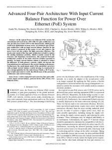
Quadrant 1: This represents a very crude modeling level that produces fast rough-cut capacity analysis, but without any AMHS details. These models are often spreadsheet modeled. As Fig. 1 explains, spreadsheet models are widely popular in capacity planning due to its ease of use and fast analysis time. However, this method does not typically yield high predictive accuracy. The modeling level described in Quadrant 2 gives a sufficiently detailed representation of the AMHS, almost to the point of emulating the actual flow of products throughout the material handling system. The problem is that these models offer little information about the production of wafers. As it is shown in the diagram in Fig. 2(a), the details of the production operations are replaced by “From–To” material flow tables, which define the rates at which materials are moved between two locations in the fab. The AMHS simulations have the following sequence: 1) a wafer lot moving between processes arrives to a “source” location (e.g., stocker, tool port); 2) the lot requests a vehicle and waits to be picked up at the “source” location; 3) an assigned vehicle travels to the “source” location to pick up the lot; 4) upon vehicle arrival, the lot is transferred into the vehicle, which then delivers the material to a “destination” location; and 5) the lot is transferred into the “destination” location, where it is terminated from the simulation. The modeling level in Quadrant 3 mimics the activities involved in the fabrication of wafers, i.e.: 1) wafers arrive to a process; 2) wait in queue for a free machine, auxiliary resource, etc.; 3) start the processing step; and 4) move to the next processing step in sequence. In the model, the details of these manufacturing activities are grouped by category (i.e., product description, stations, process description, storages, “From–To” AMHS delivery times, etc.). As it can be seen in the diagram in Fig. 2(b), these simulations provide little or no information about the AMHS. Traditionally, the modeling level in Quadrant 2 has been widely used in AMHS design, whereas the modeling level in Quadrant 3 has been popular in fab capacity planning. Most capacity planning simulations are currently run separately from AMHS design simulations. Simulating the AMHS and capacity separately often works well because the AMHS is designed to not be the bottleneck of the fab [8]. Although this approach helps maintain relatively manageable models, it is more difficult to accurately predict how the tool–AMHS interactions affect the overall fab performance. The need for predicting system performance at a higher level is the reason why the detailed levels of capacity and AMHS modeling have been combined. The models in Quadrant 4, referred herein as the capacity/AMHS model, is capable of representing and predicting the performance of the actual wafer fab and the material handling system very accurately. As one would expect, it also takes significantly longer time to simulate these models. The key to managing the size of capacity/AMHS models, and thus the execution time, is to interface the capacity model and the AMHS model efficiently. There are currently two model interfaces. In coupled capacity/AMHS models, a capacity model and an AMHS model are simulated separately and sequentially for the entire simulation and are then united by passing performance measures between them. As shown in the diagram in Fig. 2(c), the capacity model first generates

602

IEEE TRANSACTIONS ON SEMICONDUCTOR MANUFACTURING, VOL. 21, NO. 4, NOVEMBER 2008

Fig. 1. Fab modeling levels based on four different combinations of capacity and AMHS detail.

Fig. 2. Fab models at different levels of detail. (a) AMHS Model—Quadrant 2. (b) Capacity Model—Quadrant 3. (c) Coupled Capacity/AMHS Model—Quadrant 4. (d) Integrated Capacity/AMHS Model—Quadrant 4.

“From–To” material flow requirements and passes this data into the AMHS model. The AMHS model then generates and passes “From–To” delivery times into the capacity model. On the other hand, in integrated capacity/AMHS models, a capacity model and an AMHS model are combined into a single and unified simulation framework. As shown in the diagram in

Fig. 2(d), the capacity model triggers the AMHS model to execute the succeeding material handling activities that follow after a wafer completes a given production process. The AMHS model simulates the wafer delivery to the next process, and it then triggers the necessary production events in the capacity model once the lot is delivered.

JIMENEZ et al.: LEVELS OF CAPACITY AND MATERIAL HANDLING SYSTEM MODELING

603

TABLE I FACTORS THAT AFFECT LEVEL OF CAPACITY/AMHS DETAIL

B. Development of Classification Method for Levels of Fab Modeling There have been attempts to classify Fab models based on the increasing levels of capacity detail. For instance, the classification scheme presented in [9] differentiates between spreadsheets, queuing networks (QN), and simulation models. However, as was stated earlier, schemes like this do not offer sufficient information to be able to differentiate specific AMHS modeling elements. For example, they are incapable of differentiating models with simple transportation delay times and detailed representations of the interactions between wafer lots, reticles, and AMHS movements. We have extended the original concept of classification to the level of detail of the capacity component and the level of detail of the AMHS component. The classification method by the level of capacity/AMHS detail was defined by using a procedure similar to that used in [10]. In general terms, this procedure consists of two major steps: 1)

development of a preliminary classification method and 2) evaluation and modification of the preliminary method until validation issues are resolved. As a part of the development of this classification scheme, we identify the factors affecting the levels of capacity/AMHS detail, as shown in Table I. These are: modeling tool , model type , factory level , AMHS model level , capacity elements , AMHS elements , study goals , and performance metrics . We define additional subfactors within and to further specify capacity and AMHS modeling components. Note that in studies with strategic goals, decision-making has a long-term projected impact on the system (usually reflected in more than six months). Examples of studies with strategic goals include: finding number of tools, analyzing product mix, conducting ramp-up analysis, identifying bottleneck workstations, designing the AMHS, among others. On the other hand, in studies with operational goals, decision-making has a shortterm projected impact on the system (usually reflected in less

604

IEEE TRANSACTIONS ON SEMICONDUCTOR MANUFACTURING, VOL. 21, NO. 4, NOVEMBER 2008

TABLE II PROPOSED DIFFERENTIATING FACTORS FOR CAPACITY MODEL CLASSIFICATION

than six months). Examples of operational goals include: determining lot sequencing rules, evaluating scheduling rules, analyzing production operations concerning batching, setups, rework, lot sizes, reducing cycle times, and others. To develop the preliminary classification method, we analyzed approximately 30 published studies from the literature which report primarily the applications of simulation to capacity planning and AMHS design. We coded each of these studies by using a multidimensional coding scheme describing what factors and subfactors are considered in the study. See the column labeled “Codes” in Table I for a reference to the factor values. In our coding scheme, a digit and a digit represent the values taken by factor and subfactor , respectively. The collection of all digits constitutes the code. The following represents an example of how our reviewed studies are coded: Shikalgar et al. (2003).- (3, 1, 3, 1, 1, 1, 0, 1, 0, 0, 1, 1, 1, 1, 0, 1, 1, 0, 0, 0, 0, 0, 0, 0, 0, 2, 2). In the example shown above, the first four numbers describe a simulation study of the fab capacity at the factory level, but without representing the AMHS. The following 13 numbers in this code summarize the capacity components simulated, which include batching, dispatching rules, hot lots, order release poli-

cies, downtimes, secondary resources, setups, tool dedication policies, and setups. The following eight numbers indicate none of the AMHS elements are modeled. Finally, the last two numbers suggest that the study goals are strategic and the performance measure under study is cycle time. The value of the proposed coding system is that cluster analysis methodologies can be applied to discover groups of studies whose levels of detail are similar. The idea is to define the levels of capacity/AMHS detail within the preliminary classification method according to the resulting groupings. The development of the preliminary classification method is accomplished through the following Agglomerative Hierarchical Clustering Algorithm [11]. 1) Initialization: Start with groups, each containing one observation. An observation contains initially an individual simulation study. Therefore, if there are 30 studies, there are also groups. The factors affecting the level of detail are the input variables to the analysis, thus each observation has dimensions, where is the total number of factors and subfactors. Groupings are formed on the basis of similarities between input variables. As new groups are formed, observations may contain more than one study.

JIMENEZ et al.: LEVELS OF CAPACITY AND MATERIAL HANDLING SYSTEM MODELING

2) Computation of similarity matrix: An symmetric matrix is set up to indicate the similarity between pairs of groups. The similarity between two groups, say and , is given by the Euclidean distance between their -dimensional observations. 3) Combination of most similar groups in the similarity matrix (i.e., Single Linkage Method): The pair of groups with the minimum Euclidean distance is selected from the similarity matrix. These groups are combined into a new group. The similarity matrix is updated by deleting the records for the selected groups and by adding a row and column indicating the distances between the newly formed group and the remaining groups. 4) Stopping rule: Steps 2 and 3 are repeated until an adequate grouping of studies is formed. User judgment is required to interpret the levels of capacity/AMHS detail from the resulting groupings. The maximum number of repetitions times, which indicates that all studies will be in a is single group after the algorithm stops. A clustering analysis is done by using the set of factors , and (i.e., factors strongly related to the levels of capacity detail). A second clustering analysis is done , and (i.e., factors by using the set of factors related to the level of AMHS detail). Conducting two separate clustering analyses enables the development of a preliminary classification scheme with an emphasis on a combined level of capacity/AMHS detail, as proposed in Fig. 1. The results from these clustering analyses suggest that the preliminary classification method should consist of six levels of capacity detail, six levels of AMHS detail, and two levels of capacity/AMHS detail. To assure the accuracy of the final method of classification by the level of detail, further validation and modification of the preliminary method is required. The modification process is done by an analysis of an additional set of 20 studies as follows. 1) Individual studies are coded using our system for capacity/ AMHS model characteristics. 2) An individual study is assigned into one of the levels of detail. If the study does not fit in an existing category, a new level of detail is created to represent this model. Based on this validation analysis, we determined that the final classification scheme consists of six levels of capacity detail, six levels of AMHS detail, and four levels of capacity/AMHS detail. The levels of capacity detail and the levels of AMHS detail are specified in Tables II and III, respectively. We used numerical identifiers (i.e., 1-2-3-4-5-6) to represent the increasing levels of capacity detail, and alphanumerical identifiers (i.e., A-B-C-D-E-F) to represent the increasing levels of AMHS detail. The levels of capacity/AMHS detail can be divided primarily into two groups, one representing integrated models and the other representing coupled models. The factors shown in these tables represent the proposed framework for classifying fab models by level of detail. The major publications that we referenced for this study include the IEEE TRANSACTIONS ON SEMICONDUCTOR MANUFACTURING, IIE Transactions, International Journal of Production Research, Simulation, Robotics & Computer-Integrated Manufacturing, and Semiconductor International. We also referenced conference proceedings from the IEEE/SEMI Advanced Semiconductor Manufacturing Conference and the

605

TABLE III PROPOSED DIFFERENTIATING FACTORS FOR AMHS MODEL CLASSIFICATION

Winter Simulation Conference, among others. This literature review has been restricted to publications dating from 1990 to 2005. The reason for this is because the applications of AMHS to wafer fabs proliferated during this time period. III. RELATED LITERATURE REVIEW A. Current State of Literature A comprehensive list of our reviewed studies as classified with our classification method by level of capacity/AMHS detail can be found in [13]. A summary of this information is presented in Table IV. The numbers within each cell are the numbers of published articles fitting our classification scheme. This table is not intended to represent every semiconductor manufacturing study published but instead to be a representative sample. In particular, many studies are available on pure capacity models (column in Quadrant 3) that we elected not to include in our classification since they provided little additional information. A more comprehensive list of articles related to pure capacity models can be found in [14] and [15]. Some cells in Quadrant 4 contain two numbers to differentiate between the model interfaces. The first number corresponds to the number of publications using the integrated interface, and the second number corresponds to those publications using the coupled interface.

606

IEEE TRANSACTIONS ON SEMICONDUCTOR MANUFACTURING, VOL. 21, NO. 4, NOVEMBER 2008

TABLE IV CURRENT STATE OF LITERATURE ACCORDING TO CLASSIFICATION METHOD BY LEVEL OF CAPACITY AND AMHS DETAIL (I.E., 1-2-3-4-5-6 STANDS FOR LEVELS OF CAPACITY DETAIL SHOWN IN TABLE II, AND A-B-C-D-E-F STANDS FOR LEVEL OF AMHS DETAIL SHOWN IN TABLE III)

What Table IV demonstrates is a lack for tools that allow for the combination of detailed capacity models with detailed AMHS models as illustrated by the small number of studies in Quadrant 4. The major deterrents for such models are the large amount of CPU time needed to get statistically usable results and the difficulty in creating these detailed models. The remaining part of this section presents a literature review associated with and organized according to increasing levels of capacity and AMHS detail. Our review seeks to explain, in general terms, the relevant model characteristics that can potentially affect the selection of the level of detail. In Table IV, we show the current state of the literature according to the classification method by level of capacity and AMHS detail (i.e., 1-2-3-4-5-6 stands for the levels of capacity detail shown in Table II, and A-B-C-D-E-F stands for the levels of AMHS detail shown in Table III). B. Spreadsheet Capacity Models ) provide a static estiSpreadsheet models (classified as mation of the capacity of the fab by using performance metrics such as throughput and equipment efficiency. The mathematical models used within spreadsheets can be very accurate for some capacity loss agents, such as downtimes, yields, and setups [5]. Yet, capacity predictions tend to be inflated because other more complex capacity loss agents are modeled very crudely (as was shown in [9] and [16]). Despite their inaccuracy, spreadsheets are popular because they provide fast computing times, ease of use, and ease of main-

tenance [3]. This tool is often the starting point for a more complex fab modeling effort. In application, spreadsheets are often used in strategic studies, especially if the time window allocated for the project is small. In particular, these models help determine the adequate number of workstations in the fab (for example, see [17]–[19]). C. Queuing Network Models (QN) ) estimate the fab Queuing network models (classified as capacity by using time-dependent performance measures such as cycle time and work-in-progress (WIP). Unlike spreadsheets, QN models are capable of representing the variability in the system. QN models are also computational efficient. However, the capacity predictions generated with QN models can be only used as approximations because queuing models cannot capture the fab complexities accurately. QN models have been used in strategic studies, especially for rough-cut capacity analysis (for example, see [20]) and for optimizing the equipment portfolio (for example, see [21] and [22]). It is very unlikely that either spreadsheets or QN models can account for the effects of the material handling system on capacity, as the AMHS is very dynamic and complex. This can be noted by the lack of studies in this area, e.g., levels 2B-2E, 3B-3E. D. Reduced Simulation-Based Capacity (RSC) Models ) study high-utilized workstaRSC models (classified as tions without having to model the entire fab in detail. The work-

JIMENEZ et al.: LEVELS OF CAPACITY AND MATERIAL HANDLING SYSTEM MODELING

stations that add little value to total cycle time are reduced to the lowest possible detail without losing too much model accuracy. Thus, RSC models generate very accurate predictions of the CT within the workstation that is modeled in detail. In general, RSC simulations execute relatively fast, as was shown in [23]. They are also easier to update and provide a starting point for building more sophisticated simulation models [24]. In application, RSC models are used in operational studies, especially for the analysis of system bottlenecks. Most of the related literature deals with how to abstract unimportant workstations (for example, see [23] and [25]–[27]). E. Basic Simulation-Based Capacity (BSC) Models BSC models (classified as ) simulate the basic and the most representative capacity components, e.g., batching, setups, downtimes, dispatching rules, and rework. Modeling the system core with such constructs enables relatively accurate predictions of the entire fab capacity, provided that the AMHS does not cause any significant loss in capacity. However, the cycle time will be generally underestimated, especially if these estimations are compared to those produced by the capacity/AMHS model. BSC models have traditionally supported the configuration and scheduling of production processes (for example, see [28]–[30], and [31]) and also the strategic analysis of wafer fabs (for example, see [32] and [33]). F. Full Simulation-Based Capacity (FSC) Models FSC models (classified as ) have the necessary details to virtually emulate the actual fab’s production operations, thus they can predict capacity accurately. The use is suggested for configuring complex production processes, such as those processes involving complicated batching policies, lot sequencing rules, time-bound process sequences, sequence-dependent setups, reticles, etc. (for example, see [34]–[37], and [38]). The downside is the significant amount of time required to develop, validate, execute, analyze, and maintain these models. However, the time to do this is significantly less than the times required for the capacity/AMHS model.

607

the supply of AMHS vehicles is assumed infinite (i.e., level of ), the lot waiting time for vehicles can be igdetail nored. Thus, this approach helps reduce the simulation effort because “From–To” delivery times can be calculated easily, i.e., by computing delivery times as a function of distances between locations and the speed of the vehicles. Using such simple estimation of delivery time will result in very optimistic predictions of cycle time, which can then be used as lower bounds on the actual fab cycle times. The use of RSC models with AMHS time delays (classified ) has also been reported. In particular, they are used for as analyzing the operations of bottleneck workstations and for analyzing the fab and AMHS very crudely [42]. H. AMHS Models AMHS models measure key performance measures such as transport times, lot-waiting times for free vehicles, delivery times, stocker robot utilization, vehicle utilization, vehicle lost capacity, etc. AMHS models execute very slowly. However, these models produce quality predictions provided that the “From–To” material flow requirements are represented accurately [39]. Historical data or capacity models can be used to estimate material flow requirements, yet model accuracy suffers as these tools can only partially explain the AMHS dynamics [43]. Previous experimentation has also demonstrated that quality of prediction depends strongly on modeling the variability of the material flow requirements accurately by using probability distributions explaining large variance components, e.g., hyper-exponential distribution [44]. models) are used extensively AMHS models (i.e., for AMHS design. More specifically, these models are used in the design of AMHS layout (for example, see [8], [45], [46], and [47]), the analysis of the hallway transportation system (for example, see [7], [44], [48], and [49]), determination of vehicle and storage capacities (for example, see [50] and [51]), analysis of transportation technology (for example, see [52]), evaluation of vehicle control algorithms (for example, see [53]–[55]), and the analysis of AMHS delivery paradigms (for example, see [56]–[58]), among others.

G. Capacity Models With AMHS Time Delays At this level of detail, the capacity model includes a delay block to account for the transfer time of wafers between processes. These models help address the same goals as those addressed by capacity models without the AMHS construct but with higher solution quality and about the same computational effort. Experiments have shown that the CT predictions can be near to the predictions produced by the capacity/AMHS model provided that the “From–To” delivery times are represented accurately [39]. The supply of vehicles within a capacity model with AMHS time delays can be assumed to be limited (i.e., level of detail ). An assumption like this implies that data such as the time that lots spent waiting to be picked up by free vehicles has to be specified in the model. The problem with assuming a limited supply of vehicles is that lot-waiting time for vehicles can only be computed crudely through a static model, so model accuracy will suffer. Refer to [40] and [41] for examples of models within this level of detail. On the other hand, if

I. RSC/Intra-Bay AMHS Models RSC models with intra-bay AMHS models (classified as ) help analyze an entire processing area within the fab and its intra-bay AMHS. These models provide a detailed analysis of the factors affecting the tools–AMHS interactions (e.g., vehicle capacity, tool buffer capacity, process area layout, etc.), so they are therefore used widely in intra-bay AMHS design (for example, see [59] and [60]). Unfortunately, up to this point, it is unclear whether the time gains by using RSC/Intra-bay AMHS models can offset the loss in predictive quality caused by the inaccurate representations of the rest of the factory. J. Capacity/AMHS Models Capacity/AMHS models (level of detail ) contain detailed modeling constructs for the production operations, the production equipment, and the AMHS. The performance predictions produced by these models can be assumed to be representative of the actual system performance, thus managers can

608

IEEE TRANSACTIONS ON SEMICONDUCTOR MANUFACTURING, VOL. 21, NO. 4, NOVEMBER 2008

potentially make more effective decisions. These models enable higher level and integrated analysis of the equipment-AMHS interactions [61]. For example, the contributions of inter-bay AMHS technology on decreasing cycle time, delivery time, and costs were analyzed in [62] and [63]. In addition, the effect of lot sizes and priority lots on decreasing AMHS delivery times was analyzed in [64]. The problem is that it takes too long to simulate and analyze all of the desired system configurations within an integrated model. The total computational time of an integrated capacity/AMHS model is proportional to the execution time of the capacity model, the execution time of the AMHS model, and a large overhead (i.e., time to manage longer simulation lists, time to synchronize capacity model and AMHS model, etc.). To reduce the overhead times practitioners have proposed coupling a capacity model with AMHS time delays and an AMHS model. Experiments have shown that more computational efficient predictions are generated by coupling these two abstract models (for example, see [1] and [65]). However, their validity depends on using system assumptions that are consistent in both models, thus each simulation module will probably need recalibration if assumptions change. Simulation studies using coupled models include [62], [65], and [66]. IV. ANALYSIS OF CAPACITY/AMHS MODELS A. Description of Simulation Models In this section, we will attempt to demonstrate via a simulation-based abstracting methodology that coupled capacity/ AMHS models can produce system predictions that are not statistically differentiable from those produced by the integrated capacity/AMHS models. Thus, coupled models work more effectively in simulation studies with fixed budget and short analysis times, as their computational times are significantly lower than those observed by executing the detailed integrated models. Our objective in creating this methodology is to develop a fast and accurate surrogate for a fully integrated capacity/AMHS fab simulation model. It has been proposed that in many cases a queuing approximation might be a likely alternative. While we believe a queuing model might be capable of accurately predicting the cycle time of a capacity simulation, and that a similar queuing approximation might also be developed for the AMHS system, we do not see at this time how these two approximations could be combined into an accurate predictor of a fully detailed fab simulation model. This paper therefore restricts the methodological development to the improvement of simulation-based analysis methods. To carry out this experimentation, we used an existing simulation model of a 300-mm wafer fab [67]; this model is currently available at the SEMATECH website (www.sematech.org). The SEMATECH 300-mm Fab Model consists of a capacity model built in AutoSched AP [68] and an AMHS model built in AutoMod [69]. The capacity model includes ten lot types with each lot containing 25 wafers. The processing route consists of approximately 316 operations. There are 60 workstations, each workstation consisting of identical machines operating in parallel. Interruptions due to breakdowns and preventive maintenance are defined for these workstations. The time between failures

(TBF) and time to repair (TTR) are exponentially distributed. Batching, setups, and reticles are also defined for the required workstations. For planning purposes, the fab operates 24 hours per day, 365 days per year. Lots are released at a constant rate. The time between lot releases is deterministic. The AMHS model represents the machines in a 24-bay layout. There are two stockers with a capacity of 800 lots for each bay, each consisting of two input–output ports. There is a stocker robot for each stocker. There is one main transportation loop responsible for the inter-bay AMHS and 24 bay loops responsible for the intra-bay AMHS. In addition, there is one transportation loop dedicated to deliver reticles. Each bay has 24 tool positions, each consisting of two I/O ports. Number, speed, loading times, unloading times, TTR, and TBF are defined for the vehicles in each transportation loop. Users have the choice to run the SEMATECH Fab Model in one of the following modes. 1) As a separate AutoSched AP (ASAP) Capacity Model. 2) As a separate AutoMod AMHS Model. 3) As a single Integrated Model consisting of the ASAP Capacity Model and the AutoMod AMHS Model. These models are combined by using Brook’s Model Communication Module; see [70] for the details on the Model Communication Module (MCM). 4) As two Coupled Models consisting of the ASAP Model and the AutoMod Model. These models are united by using “From–To” Tables. The coupling of ASAP/AutoMod models is achieved through the following process. pilot runs are done with a pure capacity model (i.e., 1) a model without any AMHS simulation components) to approximate the “From–To” number of wafer moves. 2) The resulting “From–To” Table with the number of moves is fed into the AMHS Model. 3) pilot runs are done with the AMHS Model to produce “From–To” delivery times. 4) The resulting “From–To” Delivery Time Table is input into a delay simulation module within ASAP to simulate the AMHS activities as a black box. This forms the abstract coupled model. In this paper, pilot runs. Each “From–To” Table is thus based on the average of the five replications. It is assumed that both the number of moves and the delivery times are not stochastic, so the use of probability distributions is unnecessary. This assumption works effectively for the parameter settings used in this case study, but it could change if the coupled model is run with parameters that produce greater variability in the From–To data. B. Experimentation and Analysis To illustrate the accuracy and efficiency of abstract coupled models in relation to the detailed integrated models, we produced Cycle Time-Throughput (CT-TH) Curves for the system described above. A CT-TH curve is a tool often used by managers to determine the projected cycle time for a desired throughput level. In these curves, throughput (TH) is often represented in terms of bottleneck capacity. The relationship between bottleneck capacity and TH is empirically determined by running simulations at different points along the curve and

JIMENEZ et al.: LEVELS OF CAPACITY AND MATERIAL HANDLING SYSTEM MODELING

609

Fig. 3. Projected fab cycle times estimated by two different modeling methods.

noting utilizations of all equipment. Refer to [71] for more details concerning CT-TH curves. We produced cycle time (CT) estimates at the design points % % % and % (i.e., percent capacity of the system bottleneck that will generate a desired throughput level). Each CT point is based on ten independent replications of 100 simulation days; for each run, we cleared statistics after the first 50 days to eliminate initialization bias. The results of these simulations are depicted in Fig. 3. The points with the symbol were generated from simulation experiments using the integrated model, whereas the points with the symbol were generated from simulation experiments using a coupled model. Table V shows the relative difference and the 95% confidence intervals of the mean difference between the CT estimates produced by the coupled and integrated models (see [72] for the technical details concerning confidence intervals). Our results suggest that the coupled model and the integrated model can produce cycle time estimations that are almost identical. Because the abstraction components used within coupled capacity/AMHS models (i.e., “From–To” delivery times) will typically underestimate system variability, the loss in predictive accuracy observed by using this more abstract modeling technique increases slightly as the bottleneck utilization approaches full capacity (i.e., from 0.09% at the 70% point to 0.59% at the 97% point). However, despite such small loss of accuracy, the 95% confidence intervals indicate that we cannot statistically differentiate between coupled models and integrated models at any of the four design points.

Table V also shows the computational time in seconds that coupled models and integrated models take to run one simulation replication of 100 simulation days. These results suggest that the coupled capacity/AMHS models executes approximately 98% faster in relation to the integrated capacity/AMHS model (i.e., column f in Table V). The computational time gained by using this simulation method can significantly extend the capabilities of the experimentation. For instance, if a simulation project is allocated with the time and budget to estimate one point of the CT-TH curve with the integrated capacity/AMHS model, then we could estimate between 65 to 87 points (i.e., column g in Table V) using the coupled capacity/AMHS model within the same budget and time requirements. With this larger experimental capacity, we could analyze more system configurations by building more CT-TH curves, or we could increase the accuracy of the estimates by increasing the number of replications for each data point in the curve. The accuracy and computational efficiency observed in this case study are specific to the SEMATECH Fab Model described above. However, the SEMATECH Fab Model is a reasonably accurate model of a somewhat simplified, generic fab and even though the results do not exactly represent other fab models, similar levels of accuracy and efficiency are expected if the proposed procedures for coupling capacity/AMHS models are applied. In fact, more realistic fab models would contain greater complication and applying our approach should therefore provide even greater time reductions.

610

IEEE TRANSACTIONS ON SEMICONDUCTOR MANUFACTURING, VOL. 21, NO. 4, NOVEMBER 2008

TABLE V EXPERIMENTAL RESULTS COMPARING ACCURACY AND COMPUTATIONAL EFFICIENCY BETWEEN COUPLED MODELS AND INTEGRATED MODELS

Fig. 4. Recommended levels of modeling for integrated capacity analysis and AMHS design.

In general, the coupling modeling procedure can be applied effectively to any high-volume manufacturing system with an AMHS. It would be impractical to model the capacity system separately from the AMHS if the number of AMHS requests is nominal, as in low-volume manufacturing systems. However, the application of coupled models becomes significant as the increase of AMHS transactions affects model complexity and thus computational time. The efficiency improvements obtained with the coupled model are not exclusive to Brook’s ASAP and AutoMod. The coupled modeling procedure could be easily implemented in other simulation languages since the principle behind it is to

abstract CPU intensive modeling components into efficient and accurate simulation modules that can be easily incorporated into existing fab models. V. RECOMMENDED LEVELS OF WAFER FAB MODELING It can be assumed that refereed articles published in the literature have been carefully reviewed in terms of the capability of the simulation model to accomplish the underlying study goals efficiently and accurately. If this is the case, the published literature becomes a reliable source for determining the best matching level of capacity and AMHS modeling for typical semiconductor wafer fab problems.

JIMENEZ et al.: LEVELS OF CAPACITY AND MATERIAL HANDLING SYSTEM MODELING

611

Fig. 5. Recommended levels of modeling for pure capacity analysis.

We summarized the information provided by our literature review into the diagrams shown in Figs. 4 and 5. These flow diagrams present a series of questions that can be used to identify the requirements of the simulation study (i.e., questions are inside boxes with solid borders). These questions are followed by a recommended level of capacity and AMHS detail fitting the identified study (i.e., recommended levels of detail are inside boxes with dotted borders). The diagram in Fig. 4 attempts to recommend the levels of detail within the context of capacity analysis and AMHS design. As was demonstrated earlier in this paper, coupled capacity/AMHS models will be preferred in studies with fixed budget and time constraints because they offer the same accuracy and precision than detailed integrated models, but with greater computational efficiency. This means that using coupled capacity/AMHS models allow for more experimentation and analysis within the time allocated for the study. However, coupled capacity/AMHS models are not capable of estimating any measures describing the performance of AMHS (i.e., delivery times, AMHS utilizations, traffic congestion, etc.). For such cases, the use of detailed AMHS models is recommended. Experimentation has demonstrated that AMHS models provide results that are near to the results produced by the integrated capacity/AMHS model and the gain in computational time is significant (see [1] for more details). On the other hand, the integrated capacity/AMHS models should be used over abstractions whenever the study demands greater precision and accuracy, and at the same time, the budget and time allocated to carry out the analysis are nearly unlimited. The diagram in Fig. 5 depicts the recommended levels of detail in the context of a pure capacity analysis (i.e., the AMHS is

not modeled). For studies seeking rough approximations (e.g., within 25% of the actual value) and little computational time (e.g., less than an hour), the literature recommends using spreadsheet models if throughput, equipment utilization, availability, etc., will be measured, or QN models if cycle time and WIP need to be estimated. On the other hand, BSC models should be used instead if higher quality predictions are sought. Experimentation has shown that in some problem instances pure capacity models produce results that are approximately 15% less accurate than the integrated capacity/AMHS model (see [13] for more details). In some cases, the accuracy of BSC models is not always sufficient to estimate production performance, especially when the fab capacity is constrained by complex manufacturing processes (i.e., processes involving reticles, complicated batching policies, time-bound production sequences, etc.). For such complex system conditions, the use of FSC models is recommended, as this level of detail represents the system more accurately. VI. CONCLUSION In this paper, we described a method for classifying wafer fab models by their level of model detail. The six levels of detail of the capacity construct (i.e., material flow requirements, spreadsheet models, queuing network models, RSC models, BSC models, FSC models) and the six levels of detail of the AMHS construct (i.e., no AMHS elements, AMHS delay times with limited supply of AMHS vehicles, AMHS times with unlimited supply of AMHS vehicles, AMHS models without vehicle interference, AMHS models with vehicle interference, full AMHS model) that we proposed were developed from past published simulation studies. While it was designed for wafer

612

IEEE TRANSACTIONS ON SEMICONDUCTOR MANUFACTURING, VOL. 21, NO. 4, NOVEMBER 2008

fab systems, our classification framework by the level of detail can be applied in a more general context to other manufacturing settings, especially those that use any sort of AMHS. An extensive literature review effort indicates that sufficiently detailed fab models have not been frequently used due to the significant amount of time that it takes to run these models. This review also indicates that the use of fab model abstractions has been also very limited. The case study presented in this paper demonstrated that working with a coupled capacity/ AMHS model generated predictions that are not statistically different than those generated by a detailed integrated capacity/ AMHS model, and the savings in computational time are very significant. Thus, coupled models have been shown to be potentially efficient and accurate. It is our hope that the results obtained in this paper motivate further the development and use of abstraction methodologies. For future work, we plan to use the classification method by the level of capacity/AMHS detail in a methodology that will help model builders find an optimal abstraction level. As was discussed in [3], this work requires the development of an IP model using binary decision variables to represent whether a level of capacity/AMHS detail is selected. The objective function will minimize the total loss in result accuracy subject to constraints specifying expected project deadlines. The key for this research is to create the algorithms that will predict simulation CPU times and solution accuracy for each level of fab detail under consideration. With an optimal level of detail, it will hopefully take less time to build and execute fab models. REFERENCES [1] J. Shelton, “Fabless vision,” Future Fab Int. vol. 14, Nov. 2003 [Online]. Available: http://www.future-fab.com/documents.asp?grID=208&d_ID=1635#, [Online]. Available: [2] J. S. Pettinato, “An ITRS view on future factory integration, design, and capabilities,” Future Fab Int. vol. 16, Feb. 2004 [Online]. Available: http://www.future-fab.com/documents.asp?d_ID=3016, [Online]. Available: [3] K. Lee and P. A. Fishwick, “OOPM/RT: A multimodeling methodology for real-time simulation,” ACM Trans. Modeling and Computer Simulation, vol. 9, pp. 141–170, Apr. 1999. [4] F. Chance, J. K. Robinson, and J. W. Fowler, “Supporting manufacturing with simulation: Model design, development, and deployment,” in Proc. 1996 Winter Simulation Conf., pp. 114–121. [5] J. Robinson, J. Fowler, and E. Neacy, Capacity loss factors in semiconductor manufacturing. FabTime CA, Mar. 2003 [Online]. Available: http://www.fabtime.com/files/CapPlan.pdf, [Online]. Available: [6] G. Nadoli and D. Pillai, “Simulation in automated material handling systems design for semiconductor manufacturing,” in Proc. 1994 Winter Simulation Conf., pp. 892–899. [7] G. T. Mackulak, F. P. Lawrence, and T. Colvin, “Effective simulation model reuse: A case study for AMHS modeling,” in Proc. 1998 Winter Simulation Conf., pp. 979–984. [8] G. T. Mackulak and P. Savory, “A simulation-based experiment for comparing AMHS performance in a semiconductor fabrication facility,” IEEE Trans. Semiconduct. Manuf., vol. 14, no. 3, pp. 273–280, Aug. 2001. [9] M. Baudin, V. Mehrotra, B. Tullis, D. Yeaman, and R. A. Hughes, “From spreadsheets to simulations: A comparison of analysis methods for IC manufacturing performance,” in Proc. 1992 IEEE/SEMI Int. Semiconduct. Manuf. Science Symp., pp. 94–99. [10] N. E. Ozdemirel, G. T. Mackulak, and J. K. Cochran, “A group technology classification and coding scheme for discrete manufacturing simulation models,” Int. J. Prod. Res., vol. 31, pp. 579–601, 1993. [11] R. A. Johnson and D. W. Wichern, Applied Multivariate Statistical Analysis, 5th ed. Englewood Cliffs, NJ: Prentice–Hall, 2002, pp. 679–694. [12] R. Uzsoy, C. Y. Lee, and L. A. Martín-Vega, “A review of production planning and scheduling models in the semiconductor industry part I: System characteristics, performance evaluation and production planning,” IEE Trans., vol. 24, pp. 47–60, Sep. 1992.

[13] J. Jimenez, Simulation Modeling Levels to Support Integrated Capacity and AMHS Decision Making in Semiconductor Wafer Fabs.. Tempe: Arizona State Univ., to be published. [14] F. Chance and J. Robinson, FabTime’s Bibliography. FabTime. , CA, 2005 [Online]. Available: http://www.fabtime.com/bibliogr.shtml, [Online]. Available: [15] J. W. Fowler, J. K. Cochran, and S. M. Horng, in Abstract MASMLAB Bibliography Website. Arizona State Univ., Tempe, AZ, May 2003 [Online]. Available: http://www.eas.asu.edu/~masmlab/Biblio.html, [Online]. Available: [16] S. S. Johal, “Non-linearity and randomness in a semiconductor wafer fab,” in Proc. 1996 IEEE/SEMI Adv. Semiconductor Manufacturing Conf., pp. 17–22. [17] J. D. Witte, “Using capacity modeling techniques in semiconductor manufacturing,” in Proc. 1996 IEEE/SEMI Adv. Semiconductor Manufacturing Conf., pp. 31–35. [18] J. Neudorff, “Static capacity analysis using microsoft visual basic,” in Proc. Int. Conf. Semiconductor Manufacturing Oper. Modeling and Simulation, 1999, pp. 207–212. [19] Y.-C. Chou and R.-C. You, “A resource portfolio planning methodology for semiconductor manufacturing,” Int. J. Adv. Manuf. Technol., vol. 18, pp. 12–19, 2001. [20] H. Chen, J. M. Harrison, A. Mandelbaum, A. V. Ackere, and L. M. Wein, “Empirical evaluation for a semiconductor manufacturing wafer fabrication,” Oper. Res., vol. 36, pp. 202–215, Mar.-Apr. 1988. [21] D. P. Connors, G. E. Feigin, and D. D. Yao, “A queuing network model for semiconductor manufacturing,” IEEE Trans. Semicond. Manuf., vol. 9, no. 3, pp. 412–427, Aug. 1996. [22] W. J. Hopp, M. L. Spearman, S. Chayet, K. L. Donohue, and E. S. Gel, “Using an optimized queuing network model to support wafer fab design,” IIE Trans., vol. 34, pp. 119–130, 2002. [23] Y. F. Hung and R. C. Leachman, “Reduced simulation models of wafer fabrication facilities,” Int. J. Prod. Res., vol. 37, pp. 2685–2701, 1999. [24] Y. Shen, “Robust capacity modeling in semiconductor manufacturing,” Semiconduct. Intl. Jul. 2002 [Online]. Available: http://www.reed-electronics.com/semiconductor/index.asp?layout=article&articleid=CA231596&pubdate=7/1/2002&spacedesc=webex, [Online]. Available: [25] O. Rose, “WIP evolution of a semiconductor factory after a bottleneck workcenter breakdown,” in Proc. 1998 Winter Simulation Conf., pp. 997–1003. [26] O. Rose, “Estimation of the cycle time distribution of a wafer fab by a simple model,” in Proc. 1999 SMOMS, pp. 133–138. [27] O. Rose, “Why do simple wafer fab models fail in certain scenarios?,” in Proc. 2000 Winter Simulation Conf., pp. 1481–1490. [28] L. M. Wein, “Scheduling semiconductor wafer fabrication,” IEEE Trans. Semicond. Manuf. , vol. 1, no. 3, pp. 115–130, Aug. 1988. [29] S. Brown, F. Chance, J. W. Fowler, and J. Robinson, “A centralized approach to factory simulation,” Fut. Fab Int., vol. 1, pp. 83–86, 1997. [30] J. W. Fowler, S. Brown, H. Gold, and A. Shoeming, “Measurable improvements in cycle-time-constrained capacity,” in Proc. 1997 IEEE/ UCS/SEMI Int. Symp. Semiconductor Manufacturing, pp. 21–24. [31] M. Janakiram and J. R. Morrison, “Capacity planning and study of scheduling policies using simulation at Motorola’s ACT fab,” in Proc. Int. Conf. Semiconductor Manufacturing Oper. Modeling Simulation, 1999, pp. 201–206. [32] N. S. Grewal, T. M. Wulf, A. C. Bruska, and J. K. Robinson, “Integrating targeted cycle time reduction into the capital planning process,” in Proc. 1998 Winter Simulation Conf., pp. 1005–1010. [33] R. Stafford and J. Rimington, “Use of goal seeking for capacity analysis with semiconductor simulation models,” in Proc. Int. Conf. Semiconductor Manufacturing Oper. Modeling Simulation, 1999, pp. 213–218. [34] N. S. Grewal, T. M. Wulf, A. C. Bruska, and J. K. Robinson, “Validating simulation model cycle time at Seagate technology,” in Proc. 1999 Winter Simulation Conf., pp. 843–849. [35] L. Mönch, M. Prause, and V. Schmalfuss, “Simulation-based solution of load-balancing problems in the photolithography area of a semiconductor wafer fabrication facility,” in Proc. 2001 Winter Simulation Conf., pp. 1170–1177. [36] L. Mönch, O. Rose, and R. Sturm, “A simulation framework for the performance assessment of shop-floor control systems,” Simulation, vol. 79, pp. 163–170, Mar. 2003. [37] L. W. Schruben and T. M. Roeder, “Fast simulations of large-scale highly congested systems,” Simulation, vol. 79, pp. 115–125, Mar. 2003. [38] S. Shikalgar, D. Fronckowiak, and E. MacNair, “Application of cluster tool modeling to a 300 mm fab simulation,” in Proc. 2003 Winter Simulation Conf., pp. 1394–1397. [39] N. G. Pierce and R. Stafford, “Simulating AMHS performance for semiconductor wafer fabrication,” in Proc. 1995 Int. Symp. Semiconductor Manufacturing, pp. 165–170. [40] R. Wright, C. Cunningham, K. Benhayoune, E. Campbell, V. Swaminathan, and R. White, “300 mm factory layout and automated materials handling,” Solid State Technol., vol. 42, pp. 35–42, Dec. 1999.

JIMENEZ et al.: LEVELS OF CAPACITY AND MATERIAL HANDLING SYSTEM MODELING

[41] J. Hunter, D. Delp, D. Collins, and J. Si, “Understanding a semiconductor process using a full-scale model,” IIE Trans. Semiconduct. Manuf., vol. 15, pp. 285–289, May 2002. [42] A. Peikert, S. Brown, and J. Thoma, “A rapid modeling technique for measurable improvements in factory performance,” in Proc. 1998 Winter Simulation Conf., pp. 1011–1015. [43] S. Wu, J. Rayter, I. Paprotny, G. T. Mackulak, and J. Yngve, “Increasing first pass accuracy of AMHS simulation output using legacy data,” in Proc. 1999 Winter Simulation Conf., pp. 784–789. [44] S. Sokhan-Sanj, G. Gaxiola, G. T. Mackulak, and F. B. Malmgren, “A comparison of the exponential and the hyperexponential distributions for modeling move requests in a semiconductor fab,” in Proc. 1999 Winter Simulation Conf., pp. 774–778. [45] T. D. Colvin and G. T. Mackulak, “A concurrent engineering approach for semiconductor handling system design: A case study,” in Proc. Int. Conf. Ind. Eng. Applications, 1997, pp. 123–128. [46] T. D. Colvin, F. P. Lawrence, and G. T. Mackulak, “Soft simulation crucial for new automated fab decisions,” Solid State Technol., vol. 41, pp. 161–168, Jun. 1998. [47] T. D. Colvin, A. R. Jones, L. S. Hennessy, and G. T. Mackulak, “Fab design for 300 mm wafer handling,” Eur. Semiconduct., pp. 25–27, May 1998. [48] G. Nadoli and M. Rangaswami, “An integrated modeling methodology for material handling systems design,” in Proc. 1993 Winter Simulation Conf., pp. 785–789. [49] I. Paprotny, W. Zhao, and G. T. Mackulak, “Reducing model creation cycle time by automated conversion of a CAD AMHS layout,” in Proc. 1999 Winter Simulation Conf., pp. 779–783. [50] G. Cardarelli and P. M. Pelagagge, “Simulation tool for design and management optimization of automated interbay material handling and storage systems for large wafer fabs,” IEEE Trans. Semicond. Manuf., vol. 8, no. 1, pp. 44–49, Feb. 1995. [51] G. Cardarelli, P. M. Pelagagge, and A. Granito, “Performance analysis of automated interbay material handling and storage systems for large wafer fabs,” Robot. Comp. Integr. Manuf., vol. 12, pp. 227–234, 1996. [52] I. Paprotny, J.-Y. Shiau, Y. Huh, and G. T. Mackulak, “Simulation based comparison of semiconductor AMHS alternatives: Continuous flow vs. overhead monorail,” in Proc. 2000 Winter Simulation Conf., pp. 1333–1338. [53] N. Bahri and R. J. Gaskins, “Automated material handling system traffic control by means of node balancing,” in Proc. 2000 Winter Simulation Conf., pp. 1344–1346. [54] J. T. Lin, F.-K. Wang, and P.-Y. Yen, “Simulation analysis of dispatching rules for an automated interbay material handling system in wafer fab,” Int. J. Prod. Res., vol. 39, pp. 1221–1238, 2001. [55] M. Fukunari, S. Rajanna, R. J. Gaskins, and M. E. Sparrow, “Databased node penalties in a path-finding algorithm in an automated material handling system,” in Proc. 2002 Winter Simulation Conf., pp. 1383–1386. [56] N. Bahri, J. Reiss, and B. Doherty, “A comparison of unified vs. segregated automated material handling systems for 300 mm fabs,” in Proc. 2001 IEEE Int. Semiconductor Manufacturing Symp., pp. 3–6. [57] T. Inoue, “A comparison of AMHS delivery models in the fab of the future,” Fut. Fab Int. vol. 13, pp. 185–187, Aug. 2002 [Online]. Available: http://www.future-fab.com/documents.asp?d_ID=1319#, [Online]. Available: [58] J. T. Lin, F.-K. Wang, and C.-K. Wu, “Simulation analysis of the connecting transport AMHS in a wafer fab,” IEEE Trans. Semicond. Manuf., vol. 16, no. 3, pp. 555–564, Aug. 2003. [59] T. Jefferson, M. Rangaswami, and G. Stoner, “Simulation in the design of ground-based intrabay automation systems,” in Proc. 1996 Winter Simulation Conf., pp. 1008–1013. [60] G. T. Mackulak, F. P. Lawrence, and J. Rayter, “Simulation analysis of 300 mm intrabay automation vehicle capacity alternatives,” in Proc. 1998 IEEE/SEMI Adv. Semiconduct. Manuf. Conf., pp. 445–450. [61] R. Sturm, F. Frauenhoffer, J. Dorner, and T. Kaufmann, “Implementing manufacturing strategies for advanced capacity analysis and material handling design in the planning process of a wafer fab,” in Proc. Int. Conf. Semiconductor Manufacturing Oper. Modeling and Simulation, 1999, pp. 92–97. [62] S. Murray, G. T. Mackulak, J. W. Fowler, and T. Colvin, “A simulation-based cost modeling methodology for evaluation of interbay material handling in a semiconductor wafer fab,” in Proc. 2000 Winter Simulation Conf., pp. 1510–1517. [63] M. Schulz, T. Stanley, B. Renelt, R. Sturm, and O. Schwertschlager, “Simulation based decision support for future 300 mm automated material handling,” in Proc. 2000 Winter Simulation Conf., pp. 1518–1522. [64] S. Shikalgar, D. Fronckowiak, and E. MacNair, “300 mm wafer fabrication line simulation model,” in Proc. 2002 Winter Simulation Conf., pp. 1365–1368.

613

[65] C. D. DeJong and S. A. Fischbein, “Integrating dynamic fab capacity and automation models for 300 mm semiconductor manufacturing,” in Proc. 2000 Winter Simulation Conf., pp. 1505–1509. [66] C. D. DeJong and S. P. Wu, “Simulating the transport and scheduling of priority lots in semiconductor factories,” in Proc. 2002 Winter Simulation Conf., pp. 1387–1391. [67] SEMATECH (2002). Fab Simulation Modeling Software [Online]. Available: http://ismi.sematech.org/modeling/simulation/index. htm#models [Online]. Available: [68] “Brooks-pri automation,” in AutoSched AP 7.2 User’s Guide, Salt Lake City, UT, Oct. 2002. [69] “Brooks automation,” in AutoMod User’s Manual, Salt Lake City, UT, Mar. 2001, vol. 1–2. [70] “Brooks-pri automation,” in AutoSched AP 7.2 Customization Guide, Salt Lake City, UT, Oct. 2002. [71] J. W. Fowler, S. Park, G. T. Mackulak, and D. L. Shunk, “Efficient cycle time-throughput curve generation using a fixed sample size procedure,” Int. J. Prod. Res., vol. 39, pp. 2595–2613, 2001. [72] D. C. Montgomery, G. C. Runger, and N. F. Hubele, Eng. Stat., 3rd ed. New York: Wiley, 2004, pp. 198–260.

Jesus A. Jimenez received the B.S. and M.S. degrees in industrial engineering from The University of Texas at El Paso, El Paso, TX, in 1997 and 1999, respectively, and the Ph.D. degree in industrial engineering from Arizona State University, Tempe, AZ, in 2006. He is an Assistant Professor in the Industrial Engineering program of the Ingram School of Engineering at Texas State University-San Marcos, San Marcos, TX. His research interests are in the modeling and analysis of manufacturing systems, especially semiconductor manufacturing; automated material handling systems; the development of manufacturing applications of operations research, computer simulation, and statistics; and the reduction of time required to build, experiment, and analyze complex computer simulation models. Dr. Jimenez is member of the Institute for Operations Research and the Management Sciences (INFORMS) and the Institute of Industrial Engineers (IIE).

Gerald T. Mackulak received the B.Sc., M.Sc., and Ph.D. degrees industrial engineering, from Purdue University, West Lafayette, IN. He is an Associate Professor of Engineering in the Department of Industrial Engineering at Arizona State University. His primary area of research is simulation methodology with a focus on model abstraction, execution speed and output analysis. He has just completed work on a grant from SRC/International SEMATECH as part of the FORCE II program related to creating a simulation on demand environment. Dr. Mackulak is has received several Engineering Teaching Excellence Award nominations and is a Senior Member of the Institute of Industrial Engineering.

John W. Fowler is a Professor of Industrial Engineering at Arizona State University (ASU) and was previously the Center Director for the Factory Operations Research Center that was jointly funded by International SEMATECH and the Semiconductor Research Corporation. His research interests include modeling, analysis, and control of semiconductor manufacturing systems. Dr. Fowler is a member of IIE, INFORMS, and SCS. He is an Area Editor for SIMULATION: Transactions of the Society for Modeling and Simulation International and an Associate Editor of IEEE TRANSACTIONS ON SEMICONDUCTOR MANUFACTURING. Dr. Fowler is an IIE Fellow and is on the Winter Simulation Conference Board of Directors.