368
IEEE TRANSACTIONS ON POWER SYSTEMS, VOL. 24, NO. 1, FEBRUARY 2009
Prediction of Power System Security Levels Suad S. Halilˇcevic´, Senior Member, IEEE, Ferdinand Gubina, Life Senior Member, IEEE, and Andrej F. Gubina, Member, IEEE
Abstract—In the paper, Markov chains in conjunction with Monte Carlo simulation are used to predict the power system security level. The new approach uses a Markov chain for each identified security range to track the development of security level through time. Based on the forecasted and recorded data, the proposed procedure offers a useful tool to the system operator to predict a future power system security level. The method has been tested on the Bosnian power system using the recorded data on security levels during a one-year period. The forecasted results show a striking coincidence with the real security levels. By means of a simple and computationally fast method, the system operator can estimate the probability of a power system blackout. The presented method could be incorporated in the wide-area monitoring system in control centers. Index Terms—Markov chains, Monte Carlo simulation, prediction, security. Fig. 1. Transition between power system security state levels.
I. INTRODUCTION HE security assessment of power systems has been a serious challenge for the planners and operators, and the costs of a power system blackout are high and difficult to overcome. The power system security can be endangered by external and internal factors. The external factors encompass terrorist attacks, vandalism, ecologic impacts, while the internal factors depend on the physical nature of power system operation and on various types of contingencies. In the past, the researchers have mainly dealt with the assessment of security impact of power system component outages [1], [2]. Using a selected security index and comparing its values with the threshold values, the power system state could be classified as secure, alert or insecure in a crisp manner. The methods of artificial intelligence [3] and probabilistic techniques have also been applied to the security assessment problem [4]–[7]. These methods usually have an offline training phase used in design of prompt classifiers for an online security assessment. Some of the probability-based methods offer security assessment solutions for a single contingency, while others can be used for analysis of complex contingencies. Several studies also dealt with the online voltage security assessment [8]–[10]. Some of the studies aimed at development of methodologies for modeling security within reliability evaluation of power systems [11].
T
Manuscript received June 05, 2007; revised May 17, 2008. Current version published January 21, 2009. Paper no. TPWRS-00412-2007. S. S. Halilˇcevic´ is with the Faculty of Electrical Engineering, University of Tuzla, Tuzla, Bosnia and Herzegovina (e-mail:
[email protected]). F. Gubina and A. F. Gubina are with the Faculty of Electrical Engineering, University of Ljubljana, Ljubljana, Slovenia (e-mail:
[email protected];
[email protected]). Color versions of one or more of the figures in this paper are available online at http://ieeexplore.ieee.org. Digital Object Identifier 10.1109/TPWRS.2008.2004735
Lately, the research has focused intensively on questions related to the influence of the power market forces on system security and its assessment [12], [13]. It is very important for an operator to identify the circumstances, which could eventually endanger the power system security and to prepare for an adequate action. In [14], the software implementation has been demonstrated for an online risk-based security assessment defined in [15]. The security indices were treated as a function of existing and expected network conditions. In this paper, we focused on assessment and prediction of a power system security level. The goal was to predict the future system’s state in a probabilistic sense from the known present state. For this purpose, Markov chains are used. They may be viewed as a chain of operating states that a power system may enter, where each transition between two states is assigned an appropriate transitional probability. The Markov chain probabilistic transitional connections enable one to define the probability of a system’s transition from one operating state to another (see Fig. 1). Since each operating state has a distinct security level, the framework can describe transitions between the security levels of a power system. To describe the security level of a power system operating state, a security index must be chosen. The security index we used in the prediction describes the overall security level of the power system, the global fuzzy security index (GFSI) [16]. It compiles the security impact of all power system components encompassing generation, transmission and the segment of nodes by combining their respective fuzzy security membership grades. The GFSI is defined in such a way that it yields a measure of the fitness of the system to survive imminent disturbances without interruption of customer service, in accordance with security definition given in [17].
0885-8950/$25.00 © 2009 IEEE
ˇ ´ et al.: PREDICTION OF POWER SYSTEM SECURITY LEVELS HALILCEVIC
369
The idea of security state prediction developed in this paper is similar to the idea given in [15], where near-future security of the power system is calculated online using risk-based security indices. In contrast to [15] and other cited research, our approach uses different types of security indices and a different way of calculating the expected security levels, leading to different type of results, among them: • overall span of security level values for the system with the probabilities of their occurrence; • average value of the system security level in the near-future time frame; • probability of the lowest security level; and • probabilities of a complete and partial system blackout. In the paper we present the basic concept of the GFSI, the use of Markov chains in security prediction, the Monte Carlo simulation procedure, and the results of a case study. II. GLOBAL FUZZY SECURITY INDEX In a given operating state, each power system segment holds its own security level. In conjunction with other power system segments it influences the global security state of the power system. This approach allows for determination of the joint fuzzy security level of the power system, represented by the global fuzzy security index (GFSI). For a given operating state, the GFSI is calculated from the fuzzy security levels of the power system segments (generation, transmission, and segment of nodes). Each of these power system segments is characterized by the smallest fuzzy security membership grade (SMG) of their constitutive components. The GFSI is determined by multiplying the SMGs of the worst components (those with the lowest SMGs) of the system segments, where each segment is represented with the lowest SMG of all the components in the segment. The power system security level is then expressed as the distance between the current and the insecure operating state with the value of security index . GFSI Each component’s fuzzy security level is defined by a trapezoidal fuzzy function. It corresponds to component-specific fuzzy limits, which take into account its loading ability limits and its interaction with other power system components, including (n-1) outages of components. The fuzzy security level of a power system segment takes into account the current power system operating state . It can be as in the following: determined for chosen (1)
where S
set of the system’s operating states; SMG of an th of J components of a considered power system segment in th power system operating state; the lowest SMG of power system’s segment pss, and for power system operating state k.
Fig. 2. Interaction of power system segments in determination of the power system security.
The fuzzy operator of the right-hand side of (1) represents the minimum of the relevant SMGs. The SMG of a transmission segment results from a power flow or measured variable values with respect to their constraints of a th physical power system component ( th transmission line for instance) for a power system operating state . In a generation segment, SMG of a power reserve capacity describes the state of power reserve with respect to the defined constraints of that operating state. The GFSI varies with the operating states that the power system segments pass through, influencing the entire power system security. The interrelation of power system segment security levels is presented in Fig. 2. The SMGs are then used to calculate the GFSI, which is an aggregation of the power system segment SMGs through the fuzzy intersection operator in an operating state (2). The binary mapping is used to aggregate relevant SMGs by binary operator [18] GFSI
(2)
is the minimum value of the power system segment Here, SMGs. The GFSI describing a power system state security level can range from 0 for an insecure state, to 1 for an absolutely secure state. The proposed procedure for calculation of GFSI is presented as a block-diagram in Fig. 3, while it is investigated in detail in [16]. For each observation period, the security level as measured by GFSI is determined. The consequences of a power system operation at the opercould be severe, and the system opating state with GFSI erator must undertake adequate corrective actions. The system could experience a blackout (partial or total) following the first minor malfunction. Examples of such insecure power system , imminent state include insufficient power reserve , or certain voltage coloutage of a transmission line lapse at the next increment in load at a bus .
370
IEEE TRANSACTIONS ON POWER SYSTEMS, VOL. 24, NO. 1, FEBRUARY 2009
Fig. 5. Fuzzy membership function of bus voltage.
The fuzzy membership function of the active power reserve is a one-sided trapezoidal fuzzy set with its SMG given in the following: for for for (3)
Fig. 3. Algorithm for calculation of the GFSI.
For the segment of nodes, an example of SMG for voltage amplitude calculation is shown next. The bus voltage level fuzzy membership function and pertaining limits are defined based on the analysis of the bus voltage level deviations with its SMG shown in the following: for for for otherwise
Fig. 4. Fuzzy membership function of active power reserve.
In the generation segment, one of the defined SMGs takes into consideration an appropriate amount of power reserve, by which an emergency may be handled. The literature presents different methods of quantifying the required power reserve, mostly depending on the uncertainties that affect the power system operation. Both, the active and reactive power reserves have to be provided within the ancillary services [19]. The active power reserve (APR) necessary to stabilize the power system’s frequency is subject to the fuzzy limits (see Fig. 4). , indicates the point where the existing At active power reserve can not contribute to frequency stabilizarepresents a minimal need for tion at a disturbance and the active power reserve. The procedure to obtain such an is described in [20]. Here, the active power reserve is considered as spinning reserve. The reactive power reserve may be treated in the same way.
(4)
is set While the maximum level of the bus voltage by the insulation of the electrical equipment, the minimum bus is set as to maintain the voltage profile voltage level throughout the power system within the quality requirements. The fuzzy membership function of the bus voltage level is represented as a two-sided trapezoidal fuzzy set (see Fig. 5), where and represent the marginal values of the voltage levels that are within the required voltage range and between which . Any loading or an outage that would push the the and voltage amplitude beyond the limiting values of leads to unacceptable voltage levels. When the power system enters a new operating state, it assumes a new security level. Since the number of possible is infinite, the security states and hence security levels space is for practical application divided into n security ranges based on their values. Each range has its upper and lower margin. Each security range is then characterized by one reference security level . For all practical purposes, when describing the n security ranges, we will thus . These refwork only with n reference security levels erence levels are used in all probability distribution calculations of all security parameters for the next time period. We have conservatively selected the lower range margin as the reference security level.
ˇ ´ et al.: PREDICTION OF POWER SYSTEM SECURITY LEVELS HALILCEVIC
371
The security levels and hence the transition probabilities between them are calculated based on the recorded actual power flows. They are used to obtain a probabilistic prediction of transition for each security level from the time interval k to the next . time interval The proposed framework is flexible with regards to the number of reference security levels, which is an improvement over the traditional annotation of normal, alert and emergency [1], [2]. While each level carries a numerical value , also a descriptive labels can be used, e.g., normal, alert, insecure and emergency; by colors, or any other classification. III. MARKOV CHAINS The Markov chain is a probability chain, a discrete-time stochastic process with the Markov property. In such a process, the conditional probability distribution of a system state in the next depends only on the current state in k and time interval not on the states of previous time-periods
(5 Hence, the Markov chain describes the states of a system at successive time intervals in which the system state may change or remain the same. The change of the state is called a transition. The Markov chains are often described by directed graphs, where the edges—transitions—are labeled by transitional probabilities. In a regular Markov model, the state is directly transparent to the observer, and therefore the state transition probabilities serve as the only model parameters. The Markov chain can be based either on the first or on the th order process, depending on the number m of the previous states considered in search for the next state. For a first order transitions beprocess with M possible states, there are tween states since it is possible for any state to be succeeded state transition probabilities by another. These may be written in a state transition matrix . If the probability of the process being in a particular state at time is completely determined by the state at time k, then a Markov chain can be formed with stationary transition probabilities. Three types of Markov chains are generally used: Markov chain with stationary transition probabilities [21], [22], Markov chain based on hidden Markov model (HMM) [23]–[25], and Markov chain Monte Carlo (MCMC) [26], [27].
distribution of the n security levels of the power system. The process was modeled in discrete time intervals during which the does not vary, but it is state transition probabilities matrix changed with each MC simulation for the next time interval. The Markov chain of transitions of the security levels obtained in MC simulations are memorized and classified to one of the transitions between Markov chain nodes, i.e., between two . Each of the n of the n reference security levels Markov chains belongs to its own initial security level, identified at the beginning of the procedure. During the MC simulation, new transition probabilities are calculated for estimation of . Within the the new average security level of the system simulation, the transition from one security level to another one is randomly chosen. One MC simulation ends after a predefined number of transitions. The discrete time interval length is determined by the total time required for the three key calculations: the power flow calculation, the security level calculation, and the Monte Carlo procedure. The system security state patterns can thus be described as a Markov process characterized by and . After each MC simulation, a new transition probability matrix is obtained. Compared to the initial transition probability matrix, the new matrix has only one changed row, determined by the previous security level. With the new matrix, one can calculate the steady-state probability distribution of the security levels and in accordance with it the next expected (average) . The calculation is based on the sum system security level of products of the probabilities of the system to be in a particular security level (6) where are forecasted probabilities of security levels . After each MC simulation, the difference between the current valid and the previous forecasted average security levels is checked. When the difference is smaller than the chosen threshold the data initialization phase of security prediction cycle ends. B. State Transition Matrix The state transition matrix in the following shows an example of transition probabilities for the security ranges, represented by their reference security levels ( , , and ):
IV. MARKOV CHAIN IN SECURITY PREDICTION A. General A first order Markov process consists of the states S and state transition matrix containing transitional probabilities between security levels. The matrix describes the steady state probability vector of system security levels. For each of the n security levels, a Markov chain is constructed with a temporal series of Markov chain nodes. Since the system’s security states have an uncertain character, one may use the Monte Carlo (MC) simulation procedure as a part of the calculation procedure to estimate the next probability
(7)
If the system was previously at security level , there is a probability of 0.7 that the system stays at the same security level, 0.2 that the system could be at security level of , and probability of 0.1 that the system changes to . of initial security levels probabilities The row-vector has to be defined as in the following: (8)
372
IEEE TRANSACTIONS ON POWER SYSTEMS, VOL. 24, NO. 1, FEBRUARY 2009
In the transition defined by the first probabilistic system flucoriginates containing the probabiltuation, the new vector ities of system security levels , , and (9) In the next transition, the vector is computed again as in the following: (10) Since the associative law holds, one can write the transition probability vector of the elements (11) is the row-vector which determines transition from secuto in r iterations, when its elements become rity state declose enough to their steady-state values. The element of state notes the probability of transition from security level to security level of state in r iterations. represents the final probability distribution of the steady-state power system security levels. For the security level , the transition probabilities to other security levels of all the paths in a graph must sum to 1 (12) This concept offers an efficient prediction of the system security levels in its steady state after the process of transition described by (9)–(12).
remains with the probability 1. The system can leave the nonabsorbing state with a certain probability. The states may be rearranged so that the transition matrix can be written as a composition of four sub-matrices: , , , and (15) where the matrices describe these transition probabilities identity matrix indicating the system remaining in an absorbing state once it is reached; zero matrix representing zero probability of transition from absorbing states to non-absorbing states; transition probabilities from the non-absorbing states to the absorbing states; and transition probabilities between non-absorbing states. It is important to note that the system remains in the states of complete or partial blackout much longer than the time required for calculation of probability of the security levels. In this part of the procedure, it is necessary to determine the probability of power system to leave the state with a low security level for the state of either a complete or a partial blackout. For this purpose, the product of and matrix has to be determined. The matrix is also called the fundamental matrix, which is an inverse of the difference between the identity matrix and matrix
C. Application of Markov Chain to Security Prediction To examine a stochastic process represented by the Markov chains, one could associate them with a characterization index of power system security levels. If there are n security levels, it is interesting to trace the average probabilities that the lowest occurs, i.e., the power power system security level system enters into the dangerous state. The vector gives the probability of a power system security level dropping to the lowest (minimal) value
(13)
, the vector elements For each security level , contain the number of transitions from to the minimal secan curity level . According to [28], the expectation of be expressed as follows: (14) This way, one can compute the steady-state expected probability of the lowest power system security level, which could be an important index for a power system operator. A Markov chain has both absorbing and non-absorbing states. An absorbing state is the one in which upon entering, the system
(16) The elements of the product of and represent probabilities that the system is in one of the absorbing states of a complete or a partial system blackout. V. MONTE CARLO SIMULATION PROCEDURE The MC simulation is carried out for the Markov chain pertaining to the security levels, to which a current security level is classified. The MC procedure of the stochastic uncertainty propagation is presented in Fig. 6, as follows: . Step 1) Create a parametric model, simulaStep 2) Generate a set of random inputs, . tion of Step 3) Calculate the frequency of occurrence of security —average security level levels, matrix , and for a considered pattern of transitions, and store it as . Step 4) If , repeat steps 2 and 3 for to M (number of MC simulations); otherwise Step 5) Analyze the results using summary statistics and confidence intervals. confidence interval provides an Here, the : estimate of the accuracy of our interval estimate of , there is a 95% confidence interval; and • for • for , a 99% confidence interval is obtained. This way, we obtain the minimal and maximal values of
ˇ ´ et al.: PREDICTION OF POWER SYSTEM SECURITY LEVELS HALILCEVIC
373
Fig. 7. Uncertainty of the standard normally distributed security ranges for initial security range L .
Fig. 6. Procedure for prediction of the power system security level.
The simulation procedure calculates multiple scenarios of a model by repeatedly sampling values from the probability distributions for uncertain security levels. The MC procedure simulates possible transitions from the current, real security level to , to , and to other security levels ( to , to , if is the initial security level for the MC simulation). The number of samples taken in each of the MC simulations is assumed to be 1500. After each MC simulation, the matrix and the average security level are calculated. The MC procedure ends after the estimation error of the average of security level, as measured between two consecutive MC simulations, is less than the threshold . When the goal is achieved, one can form a new transition probability matrix and vector that are used in (11)–(15). The recorded data on actual system security levels have to be refreshed by newly identified security levels. That way, the database necessary to form the Markov chains, probability distribution functions of the security levels, and the MC simulation are updated in accordance with the actual system states. The transition probability matrix and column vector are changed after each steady state probabilities calculation until the condition: is satisfied. Each power system security level prediction pertains to one time frame k. Its length is defined by the time required for the entire calculation cycle: power flow calculation, actual security level calculation, and MC simulation. For the duration of the
time frame of a cycle, the previous actual security level is valid. At the end of the time frame, when the calculation is finished, two new security level values are obtained: the predicted average- and the actual security level. The actual security level is classified to one of the n security ranges, represented by its , and the Markov chain reference security level , pertaining to the th range is used for subsequent calculations in the next time frame of prediction. The longest calculation in the Bosnian Power System simulation took 4.5 min (Pentium IV, 3-GHz CPU). Therefore, the time frame required for security level prediction could take 4.5 min at most, which makes it quite useful for the system operator. The rule of thumb is that the more often the predictions are performed, the more valuable their results are. VI. CASE STUDY The Bosnian Power System model consists of nine P-V nodes, 20 P-Q nodes, one V- node, seven 400-kV and 28 220-kV transmission lines, and four 400/220-kV transformer substations. The time-discrete security levels are based on the actual system states recorded for the year 2004. The GFSI has been used as a measure of the security level. Assuming that the probability of the security levels was norsecurity mally distributed, we selected the following and their reference security levels : ranges
(17) The uncertainty of security levels is approximated by several discrete probability intervals as shown in Fig. 7. The standard normal distribution has been used for Monte Carlo simulation based on Sobol sampling. After the transformation of L- to z-values, the area under the normalized Gaussian Z-curve correto . sponds to the occurrence probability of security level The greater the area under the Z-curve, the higher the probability or frequency of their occurrence. These frequencies are defined by the number of the power system states transitions from one
374
IEEE TRANSACTIONS ON POWER SYSTEMS, VOL. 24, NO. 1, FEBRUARY 2009
TABLE I DATA ON SECURITY LEVEL SWITCH FOR BOSNIAN POWER SYSTEM
security level to another. There are seven discrete intervals in the case with four security ranges. In the presented case, the referhas the greatest probability of occurring, ence security level since occupies the largest area under the Z-curve. is determined The initial transition probability matrix by means of the past recorded data. Each time frame is char. The acterized by one of the reference security levels, number of distinct levels classified to one of the four security levels is normalized by the total number of time frames to determine the frequency of each security level. While the number of security ranges n can be increased, if a more precise estimation of system security is needed, this requires more computational time. The frequency of the system security transition among the different levels within a year could be determined by statistics. This information can be used to form the state transition matrix in the following and subsequently the Markov chains:
Fig. 8. Transition between security states from L1.
TABLE II BOSNIAN POWER SYSTEM SECURITY ANALYSIS FOR THREE SEGMENTS
(18)
Since the Monte Carlo procedure is applied on the Markov model, the stochastic nature of power system operation can be described. Whether the power system remains at one security level or not depends on the stochastic nature of the power system. If the new security level is classified to the same security range as the previous state’s security level, the reference security level remains the same. In Table I, the recorded data of Bosnian power system are shown. It consists of the number of instances the system has switched between two minimal security levels in 8760 observed hourly intervals, as shown in Fig. 8 from . The results of GFSI are given in Table II. The following four cases were presented for the chosen power system state in the hour 5427 in year 2004: • Case 1: operating state without outages; • Case 2: transformer outage between buses 12 and 7; • Case 3: Case 2 with start of generator in node 24 (HPP Salakovac); • Case 4: Case 2 with start of generator in node 24 and generator in node 2 (HPP Grabovica) reactive power increase. For the chosen power system state, the GFSI of 0.33 represents the security level. It belongs to the security range and its representative . Based on these data and the formed Markov chains, the procedure can start to estimate the future power system security state. The results of the MC procedure are presented in Fig. 9. The MC procedure has been calculated for 460 simulations with 1500 transition patterns of security levels
Fig. 9. MC procedure results for the initial security range of L calculated for 460 simulations of the power system security states.
for the initial reference security level . The zero values in the graph indicate the insecure states where the average security level drops to zero value, e.g., for 68th MC simulation was [0.001 0.00 0.00 0.999]. The new transition probathe bility matrix is established through the MC simulation
(19)
The initial row-vector of security level probabilities shown in (9) to (11) can be is estimated as (20)
ˇ ´ et al.: PREDICTION OF POWER SYSTEM SECURITY LEVELS HALILCEVIC
375
Fig. 11. Expected probability of the lowest security level L .
Fig. 10. Real (full line) and predicted average (short lines) security levels through the studied time.
According to (9)–(12) and (19), the predicted steady-state are shown in (21) and (22). probabilities of security levels The predicted probabilities shown in (21) arise from (21) can be expected with The results show that security level a greater probability than the other three levels , , and . . The average An average security level amounts to , security level, calculated via (6), is classified to the range represented with the reference security level . Using this procedure, the predicted transition probabilities were calculated for the other three possible reference security levels, , , and
(22) Fig. 10 presents the hourly development of the minimal predicted average security level, comparing the minimal actual security levels with the predicted data using the proposed method security ranges. The predicted average levels agree and to , except for the hours where well with the real ones, the power system security levels move to the adjacent security level. This problem could be significantly reduced if the security space was divided into more security ranges. The predicted average probability of the security level also corresponds to the actual power system security level. In Fig. 11, the expected probabilities of the lowest power system security through the studied one-year period are presented. In range order to find these probabilities, the column-vector was first calculated, containing the frequency of throughout the period (23)
Through the values in , the recorded data can be interpreted as follows: in 36% of the cases, the system is in the security range represented by and stays in that range; in 15% of cases, to , etc. In accordance with (14) the system moves from and based on one snapshot of probabilities distribution characis terized by (21), the steady-state expected probability of . The expected probability of , taking into account the possible probability distributions of all four initial security levels is 0.252, 0.246, 0.211, and 0.239. and The probability that a system with low security levels will experience a blackout (complete or partial) can be determined by the transition probability matrix .. . .. . (24) .. . .. . In accordance with (15) and (24), one can write the matrices and as in the following: and
(25)
In accordance with (16), one can write
(26) The product of and quantifies the probabilities of system and to the state of either a comsecurity transition from plete or a partial blackout. The probabilities of a system leaving security level to complete/partial blackout level are: • ; ; • ; • . • The percentage error in presented prediction is 9.8% through the whole year. Only in the time intervals between the hours
376
IEEE TRANSACTIONS ON POWER SYSTEMS, VOL. 24, NO. 1, FEBRUARY 2009
4412–4582, 4796–5280, and 5991–6198, there is a discrepancy between the real and predicted security levels. The third time frame is affected by the conservative choice of values of the predicted levels, i.e., the predicted security levels are lower than the real ones. The first two time frames of prediction are characterized by discrepancy of only one security range, e.g., in one case, while the actual bethe predicted security level belongs to longs to . The time intervals with discrepancies between the predicted and real security levels occur in periods of fast change of system’s security. A possible remedy could be a greater density of defined security ranges. When using eight instead of four ranges, the results improve and show average percentage error of 3.2% for the whole year, while the errors range from 0% to 7.5%. The possible improvements in prediction are subject of ongoing research. VII. CONCLUSION The paper presents a solution to the problem of the power system security level prediction. The approach uses the Markov chains and Monte Carlo simulation, which allow for prediction of the future power system security. Instead of assessing a power system’s security level in terms of the last disturbance only, our approach develops a multilevel security prediction, which enables the operator to foresee an effect of a disturbance in apparently normally operating power system. Moreover, the new approach makes it possible to produce a signal through the absorbing and non-absorbing states, which can be used to forestall the impending system’s blackout. The results of the new method enable the operator’s operational horizon to view a step ahead from the current power system’s state. The method proves to be simple and computationally fast, and it could be easily incorporated in the wide-area monitoring system in control centers. REFERENCES [1] C. Fu and A. Bose, “Contingency ranking based on severity indices in dynamic security analysis,” IEEE Trans. Power Syst., vol. 14, no. 3, pp. 980–987, Aug. 1999. [2] T. S. Sidhu and L. Cui, “Contingency screening for steady-state security analysis by using FFT and artificial neural networks,” IEEE Trans. Power Syst., vol. 15, no. 1, pp. 421–426, Feb. 2000. [3] M. A. Matos, N. D. Hatziargyriou, and J. A. P. Lopes, “Multicontingency steady state security evaluation using fuzzy clustering techniques,” IEEE Trans. Power Syst., vol. 15, no. 1, pp. 177–184, Feb. 2000. [4] J. W. M. Cheng, D. T. McGillis, and F. D. Galiana, “Probabilistic security analysis of bilateral transactions in a deregulated environment,” IEEE Trans. Power Syst., vol. 14, no. 3, pp. 1153–1159, Aug. 1999. [5] D. S. Kirschen, D. Jayaweera, D. Nedic, and R. N. Allan, “A probabilistic indicator of system stress,” IEEE Trans. Power Syst., vol. 19, no. 3, pp. 1650–1657, Aug. 2004. [6] Y. Dai, J. D. McCalley, N. Abi-Samra, and V. Vittal, “Annual risk assessment for overload security,” IEEE Trans. Power Syst., vol. 16, no. 4, pp. 616–623, Nov. 2001. [7] Q. Chen and J. D. McCalley, “Identifying high risk N-k contingencies for online security assessment,” IEEE Trans. Power Syst., vol. 20, no. 2, pp. 823–835, May 2005. [8] A. Berizzi, Y. G. Zeng, P. Marannino, A. Vaccarini, and P. A. Scarpellini, “A second order method for contingency severity assessment with respect to voltage collapse,” IEEE Trans. Power Syst., vol. 15, no. 1, pp. 81–88, Feb. 2000.
[9] R. A. Schlueter, S. Z. Liu, and K. Ben-Kilani, “Justification of the voltage stability security assessment and diagnostic procedure using a bifurcation subsystem method,” IEEE Trans. Power Syst., vol. 15, no. 3, pp. 1105–1112, Aug. 2000. [10] H. Lin, A. Bose, and V. Venkatasubramanian, “A fast voltage security assessment method using adaptive bounding,” IEEE Trans. Power Syst., vol. 15, no. 3, pp. 1137–1142, Aug. 2000. [11] V. A. Levi, J. M. Nahman, and D. P. Nedic, “Security modeling for power system reliability evaluation,” IEEE Trans. Power Syst., vol. 16, no. 1, pp. 29–37, Feb. 2001. [12] H. Chen, C. A. Canizares, and A. Singh, “Web-based security cost analysis in electricity markets,” IEEE Trans. Power Syst., vol. 20, no. 2, pp. 659–667, May 2005. [13] Z. Li and M. Shahidehpour, “Security-constrained unit commitment for simultaneous clearing of energy and ancillary services markets,” IEEE Trans. Power Syst., vol. 20, no. 2, pp. 1079–1089, May 2005. [14] M. Ni, J. D. McCalley, V. Vittal, S. Greene, C. W. Ten, V. S. Ganugula, and T. Tayyib, “Software implementation of online risk-based security assessment,” IEEE Trans. Power Syst., vol. 18, no. 3, pp. 1165–1173, Aug. 2003. [15] M. Ni, J. McCalley, V. Vittal, and T. Tayyib, “On-line risk-based security assessment,” IEEE Trans. Power Syst., vol. 18, no. 1, pp. 258–265, Feb. 2003. [16] S. S. Halilˇcevic´, F. Gubina, and A. F. Gubina, “The uniform fuzzy level of power system security,” Eur. Trans. Elect. Power, submitted for publication. [17] P. Kundur, J. Paserba, V. Ajjarapu, G. Andersson, A. Bose, C. Canizares, N. Hatziargyriou, D. Hill, A. Stankovic´, C. Taylor, T. Van Cutsem, and V. Vittal, “Definition and classification of power system stability,” IEEE Trans. Power Syst., vol. 19, no. 2, pp. 1387–1401, May 2004. [18] H. T. Nguyen and V. Kreinovich, “Multi-criteria optimization: An important foundation of fuzzy system design,” in Studies in Fuzzines and Soft Computing, L. Reznik, V. Dimitrov, and J. Kacprzyk, Eds. Heidelberg, Germany: Physica Verlag, 1998, Fuzzy System Design. [19] ERCOT Methodologies, ERCOT Methodologies for Determining Ancillary Service Requirements, 2001, Tech. Rep.. [20] S. Halilˇcevic´ and F. Gubina, “An on-line determination of the ready reserve power,” IEEE Trans. Power Syst., vol. 14, no. 4, pp. 1514–1520, Nov. 1999. [21] S. B. Richmond, Operations Research for Management Decision. New York: Ronald, 1968, p. 145. [22] A. M. Stankovic´ and E. A. Marengo, “A dynamic characterization of power system harmonics using Markov chains,” IEEE Trans. Power Syst., vol. 13, no. 2, pp. 442–449, May 1998. [23] R. Durbin, S. R. Eddy, A. Krogh, and G. Mitchison, Biological Sequence Analysis: Probabilistic Models of Proteins and Nucleic Acids. Cambridge, U.K.: Cambridge Univ. Press, 1999, p. 46. [24] L. Rabiner, “A tutorial on hidden Markov models and selected applications in speech recognition,” Proc. IEEE, vol. 77, no. 2, pp. 257–286, Feb. 1989. [25] J. Li, A. Najmi, and R. M. Gray, “Image classification by a two dimensional hidden Markov model,” IEEE Trans. Signal Process., vol. 48, no. 2, pp. 517–533, Feb. 2000. [26] W. R. Gilks, S. Richardson, and D. J. Spiegelhalter, Markov Chain Monte Carlo in Practice. London, U.K.: Chapman & Hall/CRC, 1996, p. 105. [27] B. A. Berg, Markov Chain Monte Carlo Simulations and Their Statistical Analysis. Singapore: World Scientific, 2004, p. 139. [28] L. Kleinrock, Queuing Systems. New York: Wiley, 1975, p. 76.
Suad S. Halilˇcevic´ (M’98–SM’06) received the B.Sc. and Ph.D. degrees from the University of Tuzla, Tuzla, Bosnia and Herzegovina, and the M.Sc. degree from the University of Zagreb, Zagreb, Croatia. He spent his research time with the Universities of Ljubljana, Dortmund (DAAD), and Aachen (DAAD). He was awarded the Fulbright scholarship at the Iowa State University in 2004–2005. He joined the Faculty of Electrical Engineering, University of Tuzla, in 1994, where he is currently an Associate Professor. He spent 11 years at the Electric Companies EP BiH, d.d. Sarajevo, and EP HZHB, d.d. Mostar. His special fields of interest are power system operation and control, and energy management.
ˇ ´ et al.: PREDICTION OF POWER SYSTEM SECURITY LEVELS HALILCEVIC
Ferdinand Gubina (M’74–LSM’04) was born in Srebrnik, Slovenia, on May 16, 1939. He received the Diploma Engineer, M.Sc., and Ph.D. degrees from The University of Ljubljana, Ljubljana, Slovenia, in 1963, 1969, and 1972, respectively. In 1970, he spent a year at the Ohio State University, Columbus, as a Fulbright Scholar and a teaching associate. Since 1988, he has been a Professor at the University of Ljubljana. His main interests lie in the area of electric power system operation and control and power planning.
377
Andrej F. Gubina (M’95) received the Diploma Engineer, M.Sc., and Ph.D. degrees from the Faculty of Electrical Engineering, University of Ljubljana, Ljubljana, Slovenia, in 1993, 1998, and 2002, respectively. In 2000, he spent a year as a Fulbright Visiting Researcher at the Massachusetts Institute of Technology, Cambridge. From 2002–2005, he headed the Risk Management Department at HSE d.o.o., Ljubljana. Since March 2007, he has headed the Laboratory for Energy Policy, and since May 2006, he has been an Assistant Professor at the University of Ljubljana. His main interests lie in the field of power system analysis and control, renewable energy sources, power market and economics, and risk management.