Leveraging Category-Level Labels For Instance-Level Image Retrieval

Leveraging Category-Level Labels For Instance-Level Image Retrieval Albert Gordoa,b∗, Jos´e A. Rodr´ıguez-Serranoa , Florent Perronnina and Ernest Valvenyb∗ a b Textual and Visual Pattern Analysis Computer Vision Center Xerox Research Center Europe, France Universitat Aut`onoma de Barcelona, Spain

Abstract

gregating them into a fixed-length vector. Within this broad framework, we can distinguish two fairly different lines of research. The first one is based on the bag-of-visual-words (BOV) framework [33] and describes an image as a very high-dimensional and very sparse histogram of visual-word counts. Retrieval efficiency is achieved through the use of inverted files. While such an approach can obtain excellent results [17, 27], it is difficult to scale to more than a couple of millions of images without dedicated hardware. The second one consists in describing images with typically smaller and denser vectors, such as the GIST [26], the Fisher vector [28, 30] or the VLAD [20], and then performing some form of encoding. It has been shown that, even with fairly small codes consisting of a few hundreds of bits, this approach could yield excellent results at a very low cost (see e.g. [38, 31, 29, 20, 12]). In this work, we follow this second line of research.

In this article, we focus on the problem of large-scale instance-level image retrieval. For efficiency reasons, it is common to represent an image by a fixed-length descriptor which is subsequently encoded into a small number of bits. We note that most encoding techniques include an unsupervised dimensionality reduction step. Our goal in this work is to learn a better subspace in a supervised manner. We especially raise the following question: “can category-level labels be used to learn such a subspace?” To answer this question, we experiment with four learning techniques: the first one is based on a metric learning framework, the second one on attribute representations, the third one on Canonical Correlation Analysis (CCA) and the fourth one on Joint Subspace and Classifier Learning (JSCL). While the first three approaches have been applied in the past to the image retrieval problem, we believe we are the first to show the usefulness of JSCL in this context. In our experiments, we use ImageNet as a source of category-level labels and report retrieval results on two standard datasets: INRIA Holidays and the University of Kentucky benchmark. Our experimental study shows that metric learning and attributes do not lead to any significant improvement in retrieval accuracy, as opposed to CCA and JSCL. As an example, we report on Holidays an increase in accuracy from 39.3% to 48.6% with 32-dimensional representations. Overall JSCL is shown to yield the best results.

We note that most encoding techniques include a projection step which is generally learned in an unsupervised manner. Our goal in this paper is to learn a better projection by leveraging labeled data to improve the retrieval accuracy for a target compression rate (or the compression rate for a target accuracy). Note that, since we learn the dimensionality reduction in a manner which is independent of a particular encoding technique, our work has the potential to impact a broad range of retrieval algorithms. An important question is the source of labeled data which we should use for supervised learning. Since our goal is to perform instance-level retrieval, it would only seem natural to use datasets labeled at the instance level. However, these datasets are typically small and as a consequence insufficient to learn a good subspace (this is shown experimentally in section 7.2). For instance, the two standard instance-level datasets we use in our experiments contain only 1,500 and 10,000 images approximately. On the other hand, there exist very large datasets of images annotated at the category-level such as ImageNet [9] which contains as of today around 14M images of 22,000 categories. Therefore, we ask in this paper the following question: can category-level labels be used to improve instance-level image retrieval?.

1. Introduction We consider the problem of query-by-example instancelevel image retrieval: given a query image of an object or a scene, we want to retrieve within a potentially large dataset other instances of the exact same object or scene. Most state-of-the-art large-scale retrieval systems consist in extracting local descriptors, such as SIFT [24], and ag∗ Albert Gordo and Ernest Valveny are partially supported by the Spanish projects TIN2009-14633-C03-03 and CONSOLIDER-INGENIO 2010 (CSD2007-00018).

1

(a)

(b)

(c)

(d)

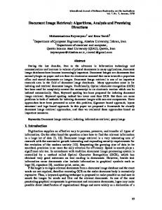
Figure 1. Results for four Holiday queries on a dataset of 1M+ images. For each query (left image), we show the top 5 retrieved images using PQ codes of 128 bits: the top row corresponds to the PCA projection baseline and the bottom row to the semantic projection with the proposed JSCL. Green frames denote correct results. See section 7 for experimental details.

This actually calls for another question: why should category-level labels help instance-level retrieval in the first place? We note that typical instance-level retrieval systems sometimes make gross mistakes, i.e. return among the top ranked results images which are visually similar but semantically unrelated. Injecting category-level information in the dimensionality reduction step should guide the retrieval system towards more semantically consistent results as shown for instance in Figure 1.

jointly learning a set of classifiers and a dimensionality reduction using a large margin framework achieves this goal. The remainder of this article is organized as follows. In the next section we review the related work. In sections 3 to 6, we describe the subspace learning approaches we experimented with: metric learning, attributes, CCA and joint classifier and subspace learning. In section 7 we compare these four algorithms on two public benchmarks.

We propose to experiment with four algorithms which learn a set of projections from labeled data. The first one is based on metric learning and casts the problem of dimensionality reduction as that of learning a low-rank Mahalanobis metric [1, 6]. Using a large margin framework, similar images are enforced to be closer in the subspace than dissimilar ones. The second one proposes to learn a set of classifiers and to represent an image as a vector of attribute scores [35, 34, 11]. The similarity between two images is then computed in this attribute space. The third one is based on Canonical Correlation Analysis (CCA) [14] and performs an embedding of labels and images in a common subspace in which the similarity can be computed [2, 12]. The fourth one consists in learning jointly a subspace and classifiers (JSCL). The classifiers are subsequently discarded and only the subspace information is used for retrieval.

2. Related Work

Our experiments show that the joint classifier and subspace learning approach performs best. For instance, in large-scale experiments on the Holidays dataset, we improve the PCA baseline from 39.3% to 48.6% for a target of 32 dimensions. Hence our two main contributions in this paper are to show (i) that category-level labeled data can be leveraged to improve instance-level retrieval and (ii) that

We now review related work in the fields which are closest to our large-scale retrieval problem – data encoding, metric learning and attribute-based retrieval – while emphasizing the differences with our own work. Data encoding. Many works have proposed to transform high-dimensional vectorial representations into compact codes. This includes Locality Sensitive Hashing (LSH) [15, 5], Spectral Hashing (SH) [38], Hamming Embedding (HE) [17], Locality Sensitive Binary Coding (LSBC) [31], Packing [18], Semi-Supervised Hashing (SSH) [36], Transform Coding (TC) [4], PCA Embedding (PCAE) [13], Iterative Quantization (ITQ) [12] or Product Quantization (PQ) [19, 20]. Despite the significant differences between these algorithms, all of them include a projection of the original image signatures into an intermediate real-valued space, as noted for instance in [13]. The projections are either random (as in LSH, LSBC, HE or Packing) or learned in an unsupervised manner, for instance with PCA (as in SH, TC, SSH, PCAE, PQ) or with an algorithm which reduces the quantization error (as in ITQ). The only work we are aware of which leverages labeled data to learn better embeddings for large-scale retrieval is that of Gong and Lazebnik

[12]. For this purpose, they propose to use CCA. This is one of the approaches we will experiment with (c.f . section 5). Note however that [12] uses category-level labels to improve category-level retrieval (also referred to as “semantic” retrieval) while we are interested in leveraging categorylevel labels to improve instance-level retrieval. Metric learning1 . Several works have proposed to leverage category-level labels to learn a similarity measure (or a distance) between two image descriptors. Note that there is a significant body of work in the machine learning community on how to “learn to retrieve” [21, 37, 1, 6, 7]. Metric learning has application to category-level image retrieval [6] but also to problems such as domain adaptation [22]. Attributes. An alternative to metric learning which has recently become popular consists in learning a set of attributes and in describing an image by a vector of attribute scores (see [23, 35, 34, 11, 8, 10, 32] among others). Again, almost all these works have considered the problem of leveraging category-level labeled data to improve category-level retrieval. A noticeable exception is the work of Douze et al. who proposed to use category-level labels to improve instance-level retrieval by fusing Fisher vectors and attributes [11]. Therefore, we will experiment with attributes in our study (c.f . section 4). However, while [11] reports a significant accuracy improvement with respect to a PCA baseline, our results are somewhat different (c.f . section 7.3).

3. Metric Learning In an image retrieval task, let q, d ∈ RD denote the D-dimensional feature vectors representing a query and a database image, respectively. We consider parametric image similarities given by the bilinear form s(q, d) = q T W d,

(1)

where W ∈ RD×D . When W = I, s(q, d) reduces to the dot-product. Instead of optimizing W directly, we consider the decomposition W = U T U , as proposed for instance in [1], where U ∈ RR×D (with R < D). Then Eq. (1) can be re-written as s(q, d) = q T U T U d = (U q)T (U d).

(2)

Eq. (2) is interesting from the point of view of data compression, since it expresses the similarity as a dot-product in a low dimensional space given by the projection matrix U . Optimizing U thus amounts to finding the linear sub-space in which the dot-product is an optimal similarity measure. A natural framework to learn U is the large margin ranking framework [1]. Given a query q, a relevant image d+ 1 In what follows,

we abuse the language and use the term “metric learning” to refer to the body of work which includes both distance and similarity learning

and an irrelevant image d− , a good similarity measure satisfies the property: s(q, d+ ) > s(q, d− ), i.e. matching pairs should have a higher similarity than non-matching pairs. Given a set of triplets (q, d+ , d− ), the goal is to minimize an upper-bound on the ranking loss: X

max{0, 1 − s(q, d+ ) + s(q, d− )}.

(3)

(q,d+ ,d− )

Since it is typically infeasible to scan all possible triplets, this loss function can be optimized using Stochastic Gradient Descent (SGD) [3]. Following straightforward derivations, it is possible to show that the training procedure consists in repeating the two following steps: (i) sample a triplet (q, d+ , d− ) randomly, and (ii) perform the gradient update U ← U + ηU (q∆T + ∆q T )

(4)

if the loss max{0, 1−s(q, d+ )+s(q, d− )} is positive, where ∆ = d+ − d− and η is the learning rate. Although the objective function (3) is not convex after the low-rank decomposition, it was shown in [1] that good results are obtained in practice by initializing the values of U randomly (from a zero-mean Normal distribution). We also experimented with an initialization from the PCA solution but this did not make a major difference. Also, following [1] we do not regularize U explicitly (e.g. by penalizing the Frobenius norm of U ) but implicitly with early stopping.

4. Attributes The principle of attribute-based representations is to describe an image with respect to a set of K “discriminative” concepts A = {a1 , . . . aK } referred to as attributes. The relevance s(q, ak ) of the image q with respect to each attribute ak is measured and the final representation is a Kdimensional vector of attribute scores: [s(q, a1 ), . . . , s(q, aK )] .

(5)

In the vast majority of cases, the attributes are learned using a large margin framework2, e.g. by training one binary Support Vector Machine (SVM) classifier for each attribute [23, 35, 34, 11, 8, 32]. If the number of attributes is smaller than the number of dimensions in the original space (a desirable property in general), then this representation can be understood as the projection of a high-dimensional representation onto a “semantic subspace”. Simple metrics, such as the dot-product of the Euclidean distance are typically used to measure the similarity within the attribute space. 2 An

exception is [10] which uses k-NN classification to measure the relevance of an image with respect to an attribute. While this approach was reported to yield excellent results for category-level retrieval, we found it to yield poor results in our instance-level retrieval scenario.

An issue with the attribute-based approach is that the dimensionality of the subspace is fixed given the number of attribute classes. However, in practice, one would like to be able to tune the dimensionality of the subspace based, for instance on a target compression factor. Douze et al. explored two simple approaches to circumvent this problem [11]. The first one consists in selecting a subset of attribute classes while the second one simply consists in applying PCA on the vector of attribute scores. Since the later approach was found to yield better results, this is the one we used in our own experiments. Note that Douze et al. also proposed to merge Fisher vectors and attribute vectors by concatenating these representations. This is an approach we will also evaluate in section 7.3.

5. Canonical Correlation Analysis Canonical Correlation Analysis (CCA) [14] is a wellknown tool for multi-view dimensionality reduction. In a nutshell, the goal of CCA is to project the multiple views into a common subspace where the correlation is maximal. Let us consider a set of N samples, and let A ∈ RDa ×N and B ∈ RDb ×N be two views of the data represented by mean-centered column feature vectors. In general, the dimensionality of the vectors in A and B are different, i.e. Da 6= Db . Let us also define the matrices Caa = AAT +ρI, T Cbb = BB T + ρI, Cab = AB T , and Cba = Cab , where ρ is a small regularization factor usually added to avoid numerically ill-conditioned situations. The goal of CCA is to find a projection of each view that maximizes the correlation between the projected representations. This can be expressed as: argmax

uT Cab v

(6)

u∈RDa ,v∈RDb

s.t.

uT Caa u = 1 and v T Cbb v = 1.

(7)

u and v are respectively the projections that embed the data from A and B into a one-dimensional common subspace where the correlation is maximal. To obtain a subspace of R dimensions we need to solve equation (6) R times to obtain the set of projections {u1 , u2 , . . . , uR } and {v1 , v2 , . . . , vR }, subject to them being uncorrelated. This can be casted as a symmetric eigenvalue problem: −1 −1 Caa Cab Cbb Cba uR = λ2R uR .

(8)

The R leading eigenvectors of equation (8) constitute the projection matrix U ∈ RR×Da used to embed A into the R-dimensional subspace. The embedding of B, if needed, can be solved analogously. In [12], CCA was used to perform supervised dimensionality reduction using respectively the image descriptors and labels as the two views. The labels were encoded as a matrix B ∈ {0, 1}K×N , where K is the number of classes,

and where Bk,n = 1 if image n belongs to category k, and 0 otherwise. In such a case, CCA can be understood as an embedding of images and labels in a common subspace.

6. Joint Subspace and Classifier Learning As is the case of CCA, we seek to embed labels and images in a common subspace. However, we wish to do so in a large margin framework. Given an image and a set of relevant and irrelevant labels, we want to enforce the relevant labels to be closer to the image in the subspace than the irrelevant ones. This process can be understood as jointly learning a set of classifiers and a dimensionality reduction. This is more optimal than learning a set of attribute classifiers and then a dimensionality reduction as in [11]. We now describe the mathematical framework. Let q be an image descriptor and let y be a category. We assume that q ∈ RD and that there are K categories, i.e. y ∈ {1, . . . , K}. Let us measure the relevance of y with respect to q (i.e. the score of class y on q) as follows: s(q, y) = (U q)T wy

(9)

where U ∈ RR×D matrix which projects q in a R dimensional subspace (with R < D and R ≤ K) and wy is the classifier of class y in the low-dimensional space. Hence, the projection matrix U is shared across all classes. Given a set of triplets (q, y + , y − ) where y + is relevant to q and y − is irrelevant to q (i.e. q is labeled with y + but not with y − ), we minimize an upper-bound on the label ranking loss: X  max 0, 1 − s(q, y + ) + s(q, y − ) (10) (q,y + ,y − )

Weston et al. proposed a similar objective function in [16] for annotation purposes. In what follows, we choose to optimize equation (10) because it is more similar to the metric learning framework of [1] that we use as a baseline and therefore, it offers a fairer comparison. Note that we also ran experiments with the objective function proposed by Weston et al. and we found it to yield very similar results. As was the case for metric learning, this objective function can be optimized with SGD by sampling a triplet (q, y + , y − ). If the loss max {0, 1 − s(q, y + ) + s(q, y − )} is positive, then the following update rules are applied: U wy+ wy−

← U + η(wy+ − wy− )q T

(11)

← wy+ + ηU q ← wy− − ηU q

(12) (13)

where η is again the learning step size. As was the case for metric learning, we initial the matrix U randomly (from a zero-mean Normal distribution). and use early stopping for regularization. After learning, we discard the classifiers wy and keep only the projection matrix U .

7. Experimental validation We first describe the datasets and features we used in our experiments. We then provide results for the metric learning and attribute-based approaches. Finally, we present results for the two label-image embedding techniques: CCA and joint classifier and subspace learning.

7.1. Datasets and features Datasets. We use the two following public benchmarks for evaluation. INRIA Holidays3 [17] contains 1,491 images of 500 scenes and objects. One image per scene / object is used as query to search within the remaining 1,490 images and accuracy is measured as the Average Precision (AP) averaged over the 500 queries (mAP). The University of Kentucky Benchmark (UKB)4 [25] contains 10,200 images of 2,550 objects. Each image is used in turn as query to search within the 10,200 images and accuracy is measured as 4×recall@4 averaged over the 10,200 queries. Hence, the maximum achievable score is 4 on this dataset. We use the ImageNet Large Scale Visual Recognition Challenge (ILSVRC) 2010 dataset5 for learning purposes. We use it both for unsupervised learning (e.g. to learn a PCA) and for supervised learning (e.g. to learn a metric, attributes, CCA, etc.) This dataset contains 1,000 classes and consists of 3 sets: a training, a validation and a test set. In our experiments, we only make use of the training set which contains 1.2M images. For the large-scale experiments reported in Section 7.4, we also use a subset of 1M ImageNet images to serve as distractors. They were randomly sampled from the full ImageNet dataset [9] (excluding the ILSVRC 2010 categories) Features. We extract 128-dimensional SIFT descriptors [24] and 96-dimensional color descriptors [30] on regular grids at multiple scales. Contrarily to most previous instance-level retrieval works, we do not make use of interest-point detectors. We found dense extraction to yield somewhat better (resp. worse) results on Holidays (resp. UKB). Note however that this saves the interest-point detection time which is substantial in our large-scale experiments. These features are reduced to 64 dimensions with PCA. We compute separately for each descriptor a 2,048dimensional Fisher Vector (FV) which is power- and L2normalized [29, 30]. The SIFT and color FVs are subsequently concatenated, thus yielding a 4,096-dim image descriptor. The distance between two FVs is computed with a dot-product [29]. This provides a baseline of 77.4% on Holidays and 3.19 on UKB. 3 http://lear.inrialpes.fr/

˜jegou/data.php ˜stewe/ukbench/ 5 http://www.image-net.org/challenges/LSVRC/2010 4 http://www.vis.uky.edu/

Figure 2. First row: random images from the ImageNet category n02930766 (“cab, hack, taxi, taxicab”). Second row: n03786901 (“mortar”). Third row: n04147183 (“Schooner”). R= PCA IL CL

16 53.1 52.1 36.8

32 61.3 62.9 54.2

64 68.0 67.1 65.1

128 72.3 73.2 68.9

256 75.0 75.8 75.4

512 76.8 77.1 78.6

Table 1. Subspace learning as metric learning. Results on Holidays (mAP, in %) when learning with Instance Level (IL) and Category Level (CL) labels. R= PCA IL CL

16 2.56 1.09 1.80

32 2.82 1.99 2.37

64 3.01 2.55 2.78

128 3.08 2.90 2.95

256 3.15 3.07 3.09

512 3.18 3.16 3.16

Table 2. Subspace learning as metric learning. Results on UKB (4× recall@4) when learning with Instance Level (IL) and Category Level (CL) labels.

7.2. Results with metric learning When learning a metric for a target subspace dimension R, two parameters need to be tuned: the step size η as well as the number of iterations niter. We performed two sets of experiments. In the first set of experiments we learn the subspace from ILSVRC 2010. To avoid tuning η and niter on the test data, we validated our Holidays results on UKB and vice versa, i.e. we report results on Holidays (resp. UKB) with the parameters that lead to the best results on UKB (resp. Holidays). This shows the ability of the learning algorithm to generalize to new data. In the second set of experiments, we learn the subspace from instance-level labels. For the Holidays experiments, we therefore trained the subspace on UKB and vice-versa. In this set of experiments, η and niter were tuned directly to maximize test accuracy which gives an unfair advantage to this approach. The metric learning results are reported in Tables 1 and

FV (4,096 dim) Attr (1,000 dim) FV + Attr (5,096 dim)

Holidays 77.4% 76.2% 78.1%

UKB 3.19 3.27 3.27

Table 3. Combining FVs and attributes. Results on Holidays (mAP, in %) and UKB (4× recall@4).

2 and compared to the PCA baseline. We can draw the two following conclusions. First, metric learning with instancelevel labels (IL) does not significantly improve accuracy on Holidays or UKB. It is actually significantly worse than the PCA baseline on UKB. We believe this is because the training datasets (UKB for Holidays and Holidays for UKB) are too small to learn a meaningful subspace. Note that we are not aware of any significantly larger dataset with instancelevel labels. Second, metric learning on category-level labels (CL) yields poor results, especially for a small number of dimensions R. We observe a small improvement with respect to the PCA baseline on Holidays for a larger R (e.g. R = 512). Our intuition to explain these poor results is the following one: although images within the same category might be visually dissimilar (c.f . Fig 2), metric learning tries to enforce them explicitly to be closer to each other than to images in other categories.

7.3. Results with attributes To learn the attribute classifiers, we first extract from the 1.2M ILSVRC 2010 training images the same 4,096dimensional FV features we use for retrieval (c.f . section 7.1). We then learn 1,000 one-vs-all binary linear SVMs using SGD6 . Note that learning classifiers on FVs makes sense as shown for instance in [30]. Given an image, we construct its attribute vector by concatenating the 1,000 classifier scores, which yields a 1,000-dimensional vector. Hence, the computation of the attribute scores can be understood as a linear projection in a 1,000-dimensional subspace. The attribute vector is subsequently L2-normalized and we use the dot-product as a measure of similarity. Following [11], we also report results combining the FV and the attributes. As suggested by [11], we apply a weighting factor to increase the contribution of the FV. To avoid tuning this parameter on the test data, the optimal weight for Holidays (resp. UKB) was cross-validated on UKB (resp. Holidays). Results are reported in Table 3. We observe that attributes perform slightly worse than FVs on Holidays and slightly better on UKB. We also note that there seems to be little complementarity between FVs and attributes. Since our focus is on subspace learning, we also perform dimensionality reduction by applying PCA to the FV and the attributes independently and by concatenating the resulting vectors, as suggested in [11]. To produce a sig6 http://leon.bottou.org/projects/sgd

R= FV FV + Attr

16 53.1 49.3

32 61.3 60.3

64 68.0 66.4

128 72.3 71.2

256 75.0 75.2

512 76.8 76.8

Table 4. Combining FVs and attributes after PCA. Results on Holidays (mAP, in %).

nature of R dimensions, FVs and attributes are reduced to R/2 dimensions and concatenated. Again, we tune the relative weight of the FV part with respect to the attribute part. Table 4 compares this approach with the PCA baseline on the Holidays dataset and we observe no improvement. These results somewhat contradict those of [11] who reported a significant improvement on Holidays when merging FVs and attributes. We believe this is because the features used by [11] to learn the attributes contained information not available in the FV. For instance, their attributes used, among others, color information, while their FVs were computed from SIFT descriptors only. To test this conjecture, we computed 2,048-dimensional FVs using only SIFT descriptors as well as 1,000-dimensional attribute vectors computed from color-only descriptors. Combining the FV and attributes in this case makes a significant difference on Holidays: from 68.5.% using SIFT FVs (2,048 dimensions) to 76.2% when concatenating SIFT FVs and color attributes (3,048 dimensions). We believe this experiment validates our point. Note that we can obtain a similar accuracy of 76.8% in a simple manner, by reducing the dimensionality of the 4,096-dimensional SIFT+color FV to 512 dimensions. Our conclusion is therefore that attributes do not seem to improve instance-level retrieval significantly on these datasets.

7.4. Results with label-image embedding We now report results for those two approaches which perform an embedding of images and labels in a common subspace: CCA and the proposed Joint Subspace and Classifier Learning (JSCL). For both the CCA and JSCL, we use again ILSVRC 2010 for learning. For CCA, there is a single parameter to tune: the regularization parameter ρ (c.f . section 5). As for JSCL, there are two parameters to tune (as was the case for metric learning): the step size η and the number of iterations niter. As was the case in our previews experiments, to avoid tuning the parameters on the test data, we validate the Holidays (resp. UKB) parameters on UKB (resp. Holidays). We report results on Holidays in Table 5 and UKB in Table 6. We can make the two following observations. First, both label-image embedding methods improve over the PCA baseline, especially for a small number of dimensions R of the subspace (e.g. R = 32). Second, JSCL generally yields better results than CCA. This seems to indicate that using a

R= PCA CCA JSCL

16 53.1 54.5 56.7

32 61.3 62.9 67.7

64 68.0 71.0 73.6

128 72.3 74.7 76.4

256 75.0 77.6 78.3

512 76.8 79.0 78.9

80 70

R= PCA CCA JSCL

16 2.56 2.52 2.67

32 2.82 2.90 3.04

64 3.01 3.11 3.23

128 3.08 3.22 3.31

256 3.15 3.29 3.36

512 3.18 3.32 3.36

mAP (in %)

60

Table 5. Results of CCA and the proposed JSCL as compared to the PCA baseline on Holidays (mAP, in %).

50 40 PCA CCA JSCL PCA + PQ CCA + PQ JSCL + PQ

30 20 10

Table 6. Results of CCA and the proposed JSCL as compared to the PCA baseline on UKB (4× recall@4).

32

64

128

256

512

Number of Dimensions 3.5

3 4 x Recall at 4

large margin framework enables to uncover a more discriminative subspace. On UKB, we point out that we can both reduce the dimensionality of the initial 4,096-dimensional FV representation down to 256 dimensions and increase the retrieval accuracy from 3.19 to 3.36. Since our focus is on large-scale retrieval, we also performed an evaluation with a large set of distractor images as is common practice (see e.g. [17, 27, 20, 11]). In our experiments, we use 1M ImageNet images (c.f . section 7.1). Hence, when running a search on Holidays (resp. UKB), the system compares the query to the 1,490 (resp. 10,200) database images + 1M distractors. We ran two sets of experiments. In the first set of experiments, the dimensionality of the FV is reduced (through PCA, CCA or JSCL) but no further compression is applied. In the second set of experiments, the dimensionality of the FV is reduced and a Product Quantization (PQ) [19] is further applied to encode the descriptors. We chose PQ since it yields state-of-the-art codes when combined with dimensionality reduction [20] but other encoding techniques could have been applied too. In a nutshell, PQ splits the large FV into small sub-vectors and applies a separate Vector Quantizer (VQ) to each subvector independently (see [19] for more details). In our experiments we use sub-vectors of 8 dimensions and each subvector is encoded on 8 bits. Hence, with such a configuration, if PQ takes as input a K-dimensional vector, it outputs a K bits code. Results for Holidays and UKB are presented in Fig. 3. We can draw the following conclusions. As in the case of small-scale experiments, CCA and JSCL improve over PCA. Moreover, JSCL seems to have an edge over CCA. These observations are valid whether PQ encoding is applied or not. The differences with the PCA baseline seem more acute in large-scale experiments than in small-scale experiments. For instance, the retrieval accuracy is improved from 39.3% with PCA to 48.6% with JSCL with R = 32 (without compression) on Holidays. This seems to indicate that learning good projections has a larger impact

2.5

PCA CCA JSCL PCA + PQ CCA + PQ JSCL + PQ

2

1.5 32

64

128

256

512

Number of Dimensions

Figure 3. Large-scale results of CCA and the proposed JSCL as compared to the PCA baseline. Top: Holidays + 1M distractors (mAP in %). Bottom: UKB + 1M distractors (4× recall@4).

for more complex problems, e.g. when the relevant images are lost in a sea of irrelevant ones. Finally, Figure 1 shows qualitative results on Holidays+1M using PQ codes of 128 bits. We show the top 5 results on 4 queries and compare the PCA and JSCL embeddings. The queries have been chosen such as that there is no intersection between the top PCA and JSCL results. We observe how the JSCL results are semantically more consistent than those of PCA, even if sometimes PCA finds true positives that JSCL misses, such as that of 1d.

8. Conclusion At the beginning of this article, we raised the following question: can category-level labels be used to improve instance-level image retrieval? We can now answer this question positively. To reach this conclusion, we experimented with four learning techniques: the first one is based on a metric learning framework, the second one on attribute representations, the third one on Canonical Correlation Analysis (CCA) and the fourth one on Joint Sub-

space and Classifier Learning (JSCL). While the first three approaches had been applied to some extent to the image retrieval problem in the past, we believe we are the first to show the usefulness of JSCL in this context. Our experimental evaluation showed that metriclearning and attributes do not improve significantly over the baseline system. In some cases, it can even lead to a decrease in accuracy. We also showed that CCA and JSCL, which both consist in embedding labels and images in a common subspace, can lead to substantial improvements, especially in large-scale experiments. Overall, JSCL yields the best results and we believe that it superiority with respect to the simpler CCA approach comes from the use of a large margin formulation. Thus, a key conclusion of our work is that one might get a superior performance with a method such as JSCL which optimizes a categorization objective function (which is consistent with the category-level labels we use for training but which is only loosely consistent with our retrieval objective) than with a method such as metric learning which optimizes a retrieval objective function (which is consistent with our instance-level retrieval problem but which is inconsistent with our category-level labels). We finally note that those methods which jointly embed labels and images in a common subspace, such as CCA and JSCL, have an additional advantage which we have not exploited in this work. Indeed, since labels and images have a common representation, one could easily perform query-by-example and query-by-text searches within a unified framework. We will explore the advantages of such an approach in future work.

References [1] B. Bai, J. Weston, D. Grangier, R. Collobert, K. Sadamasa, Y. Qi, O. Chapelle, and K. Weinberger. Supervised semantic indexing. In CIKM, 2009. 2, 3, 4 [2] M. Blaschko and C. Lampert. Correlational spectral clustering. In CVPR, 2008. 2 [3] L. Bottou. Stochastic learning. In Advanced Lectures on Machine Learning, 2003. 3 [4] J. Brandt. Transform coding for fast approximate nearest neighbor search in high dimensions. In CVPR, 2010. 2 [5] M. Charikar. Similarity estimation techniques from rounding algorithms. In ACM STOC, 2002. 2 [6] G. Chechik, U. Shalit, V. Sharma, and S. Bengio. An online algorithm for large scale image similarity learning. In NIPS, 2009. 2, 3 [7] J. V. Davis, B. Kulis, P. Jain, S. Sra, and I. S. Dhillon. Informationtheoretic metric learning. In ICML, 2007. 3 [8] J. Deng, A. Berg, and L. Fei-Fei. Hierarchical semantic indexing for large scale image retrieval. In CVPR, 2011. 3 [9] J. Deng, W. Dong, R. Socher, L.-J. Li, K. Li, and L. Fei-Fei. Imagenet: A large-scale hierarchical image database. In CVPR, 2009. 1, 5 [10] T. Deselaers and V. Ferrari. Visual and semantic similarity in imagenet. In CVPR, 2011. 3

[11] M. Douze, A. Ramisa, and C. Schmid. Combining attributes and fisher vectors for efficient image retrieval. In CVPR, 2011. 2, 3, 4, 6, 7 [12] Y. Gong and S. Lazebnik. Iterative quantization: A procrustean approach to learning binary codes. In CVPR, 2011. 1, 2, 3, 4 [13] A. Gordo and F. Perronnin. Asymmetric distances for binary embeddings. In CVPR, 2011. 2 [14] H. Hotelling. Relations between two sets of variates. Biometrika, 1936. 2, 4 [15] P. Indyk and R. Motwani. Approximate nearest neighbors: towards removing the curse of dimensionality. In ACM STOC, 1998. 2 [16] S. B. J. Weston and N. Usunier. Large scale image annotation: learning to rank with joint word-image embeddings. In ECML, 2010. 4 [17] H. J´egou, M. Douze, and C. Schmid. Hamming embedding and weak geometry consistency for large scale image search. In ECCV, 2008. 1, 2, 5, 7 [18] H. J´egou, M. Douze, and C. Schmid. Packing bag-of-features. In ICCV, 2009. 2 [19] H. J´egou, M. Douze, and C. Schmid. Product quantization for nearest neighbor search. IEEE TPAMI, 2011. 2, 7 [20] H. J´egou, M. Douze, C. Schmid, and P. P´erez. Aggregating local descriptors into a compact image representation. In CVPR, 2010. 1, 2, 7 [21] T. Joachims. Optimizing search engines using clickthrough data. In KDD, 2002. 3 [22] B. Kulis, K. Saenko, and T. Darrell. What you saw is not what you get: Domain adaptation using asymmetric kernel transforms. In CVPR, 2011. 3 [23] C. Lampert, H. Nickisch, and S. Harmeling. Learning to detect unseen object classes by between-class attribute transfer. In CVPR, 2009. 3 [24] D. Lowe. Distinctive image features from scale-invariant keypoints. IJCV, 2004. 1, 5 [25] D. Nist´er and H. Stew´enius. Scalable recognition with a vocabulary tree. In CVPR, 2006. 5 [26] A. Oliva and A. Torralba. Modeling the shape of the scene: a holistic representation of the spatial envelope. IJCV, 2001. 1 [27] M. Perd´och, O. Chum, and J. Matas. Efficient representation of local geometry for large scale object retrieval. In CVPR, 2009. 1, 7 [28] F. Perronnin and C. Dance. Fisher kernels on visual vocabularies for image categorization. In CVPR, 2007. 1 [29] F. Perronnin, Y. Liu, J. S´anchez, and H. Poirier. Large-scale image retrieval with compressed fisher vectors. In CVPR, 2010. 1, 5 [30] F. Perronnin, J. S´anchez, and T. Mensink. Improving the Fisher kernel for large-scale image classification. In ECCV, 2010. 1, 5, 6 [31] M. Raginsky and S. Lazebnik. Locality-sensitive binary codes from shift-invariant kernels. In NIPS, 2009. 1, 2 [32] M. Rastegari, C. Fang, and L. Torresani. Scalable object-class retrieval with approximate and top-k ranking. In ICCV, 2011. 3 [33] J. Sivic and A. Zisserman. Video Google: A text retrieval approach to object matching in videos. In ICCV, 2003. 1 [34] L. Torresani, M. Szummer, and A. Fitzgibbon. Efficient object category recognition using classemes. In ECCV, 2010. 2, 3 [35] G. Wang, D. Hoiem, and D. Forsyth. Learning image similarity from Flickr groups using stochastic intersection kernel machines. In ICCV, 2009. 2, 3 [36] J. Wang, S. Kumar, and S.-F. Chang. Semi-supervised hashing for large scale search. In CVPR, 2010. 2 [37] K. Weinberger and L. Saul. Distance metric learning for large margin nearest neighbor classification. JMLR, 2009. 3 [38] Y. Weiss, A. Torralba, and R. Fergus. Spectral hashing. In NIPS, 2008. 1, 2