LGH: A Fast and Accurate Algorithm for Single ...

JOURNAL OF LATEX CLASS FILES, VOL. 6, NO. 1, JANUARY 2014

1

LGH: A Fast and Accurate Algorithm for Single Individual Haplotyping Based on a Two-Locus Linkage Graph Minzhu Xie, Jianxin Wang, Senior Member, IEEE, and Xin Chen Abstract—Phased haplotype information is crucial in our complete understanding of differences between individuals at the genetic level. Given a collection of DNA fragments sequenced from a homologous pair of chromosomes, the problem of Single Individual Haplotyping (SIH) aims to reconstruct a pair of haplotypes using a computer algorithm. In this paper, we encode the information of aligned DNA fragments into a two-locus linkage graph and approach the SIH problem by vertex labeling of the graph. In order to find a vertex labeling with the minimum sum of weights of incompatible edges, we develop a fast and accurate heuristic algorithm. It starts with detecting error-tolerant components by an adapted breadth-first search. A proper labeling of vertices is then identified for each component, with which sequencing errors are further corrected and edge weights are adjusted accordingly. After contracting each error-tolerant component into a single vertex, the above procedure is iterated on the resulting condensed linkage graph until error-tolerant components are no longer detected. The algorithm finally outputs a haplotype pair based on the vertex labeling. Extensive experiments on simulated and real data show that our algorithm is more accurate and faster than five existing algorithms for single individual haplotyping. Index Terms—Single individual haplotyping, next-generation sequencing, error correction, algorithm.

F

1

I NTRODUCTION

B

EING a diploid creature, a human being has two copies of each chromosome with one from father and another from mother. Though the two copies are very similar, there are about 0.5% differences between them [1]. Despite many advances in DNA sequencing technologies, it is still labor-consuming and expensive to separate the two homologous copies of a chromosome for sequencing individually [2], [3]. Most published human genome sequences provide only the mixed allele information of the underlying two copies of chromosomes [4]. However, the variants combination information along a chromosome (i.e., haplotype) is crucial in the complete understanding of human complex genetic polymorphisms. Increasing evidence shows that phenotypic effects of genomic variants can be better understood with haplotypes rather than isolated variants, and that haplotypes can enhance the power of genome-wide association studies for complex diseases [5], [6]. Therefore, computational approaches are needed to infer the underlying haplotypes from the mixed allele information of • corresponding authors: Minzhu Xie and Xin Chen. E-mail: [email protected]; [email protected] • M. Xie and X. Chen are with School of Physical and Mathematical Sciences, Nanyang Technological University, 637371, Singapore. • M. Xie is with College of Physics and Information Science, Hunan Normal University, Changsha, 410081, China. • Jianxin Wang is with School of Information Science and Engineering, Central South University, Changsha, 410083, China.

genotype data. Many computational haplotyping algorithms [7], [8], [9] have been proposed and they mainly fall into two categories: population haplotyping (also called haplotype inference) and single individual haplotyping (SIH) [10]. Population haplotyping tries to build haplotypes from the genotype data of a sample of individuals in a population. However, it is unable to recognize rare or novel variants. Moreover, for a population sample from unrelated individuals, genotype information is generally not sufficient for an accurate inference of the haplotype pattern in a large region (>100 kbp) [7]. SIH is also called haplotype assembly. Given a set of DNA fragments sequenced from a homologous pair of chromosomes of an individual, SIH aims to reconstruct a pair of haplotypes of the underlying chromosomes after aligning the fragments to a reference sequence. Even at medium fragment coverage on heterogeneous variant loci, SIH often builds longer and more accurate haplotype blocks than population haplotyping [11]. With matepair sequencing and read length improvements of sequencing technologies, SIH has become a practical approach for haplotype reconstruction in personal genome sequencing [12], [13]. For instance, a recent study [14] showed that 99% of single-nucleotide variants in human genomes can be phased into haplotype blocks of length 0.2-1 Mbp using long-range PCR and single individual haplotyping. However, the presence of sequencing errors in DNA fragments makes the SIH problem very difficult. To

JOURNAL OF LATEX CLASS FILES, VOL. 6, NO. 1, JANUARY 2014

deal with sequencing errors, previous studies have proposed many SIH computational models and algorithms. Lancia et al. [15] first introduced the SIH problem together with three optimization models: minimum fragment removal (MFR), minimum SNP removal (MSR) and longest haplotype reconstruction (LHR). A model of special interest is minimum error correction (MEC) [16], which aims to reconstruct haplotypes by correcting as few errors in the fragments as possible. Recently, Duitama et al. proposed a model called maximum fragments cut (MFC) [17], and Xie et al. proposed a model called balanced optimal partition (BOP) by combining two measures “errors corrected” and “fragments cut” [18]. If there are additional data such as genotypes and reference haplotypes available, some extended models [19], [20] and frameworks [21], [22] can be used to phase a pair of haplotypes of an individual. Note that most of the above optimization problems are NP-hard [15], [16]. As a result, their exact algorithms may require a formidable amount of running time so that they become impractical for some real datasets [23], [24], [25], [26]. To obtain an efficient solver, a number of heuristic algorithms have been designed [17], [18], [19], [27], [28]. As reported, HapCut [7], ReFHap [17] and H-BOP [18] are among the fastest and most accurate heuristic algorithms which take only aligned fragments as input data. In this paper, we encode the information of DNA fragments covering two or more heterozygous variant loci into a two-locus linkage graph, where each vertex represents a variant locus and an edge is associated with the information of combinatorial patterns of variants at two loci. Then we approach the SIH problem by finding a vertex labeling of the graph with the minimum sum of weights of all incompatible edges.

2 2.1

M ETHODS Formulation and Problem

A single nucleotide polymorphism (SNP) is a single nucleotide variation at a given locus of a genome sequence. SNPs are the dominant type of human genetic variations, and millions of SNPs have been validated distributing throughout the human genome. Here we consider a haplotype as the sequence of SNPs on a chromosome in a given region and, moreover, consider only the alleles at those SNP loci covered by the input aligned fragments. It is commonly assumed that human SNPs have only two possible alleles at a locus, under which we represent the major allele (the more common or frequent allele in a population) as ‘0’ and the minor allele as ‘1’. Hence, both haplotypes and the input aligned fragments can be encoded as strings over a three-letter alphabet {0, 1, −}, where ‘−’ denotes an unknown allele. We use f to denote a fragment and h to denote a haplotype, while h[i] and f [i] denote the ith character of h and f , respectively. Since a

2

fragment covering only one heterozygous SNP locus would not help resolve haplotyping and, on the other hand, determining the alleles of a haplotype pair at homozygous SNP loci is trivial, we assume below that all SNP loci are heterozygous and that every input fragment covers at least two heterozygous SNP loci. Thus, for a haplotype pair H = {h1 , h2 }, h1 and h2 shall be bit-wise complementary to each other, i.e., if h1 [i] = 0 then h2 [i] = 1, and if h1 [i] = 1 then h2 [i] = 0. Without loss of generality, we further assume h1 to be the haplotype in H that starts with 0. When a pair of haplotypes are restricted to two heterozygous loci, there are only two different combinatorial patterns: (i) one haplotype is seen as “0 0” and another as “1 1”; (ii) one haplotype is “0 1” and another is “1 0”. The first pattern is denoted by “0 0 / 1 1” and the second by “0 1 / 1 0”. For a fragment covering l (l ≥ 2) SNP loci, we can obtain the combinatorial pattern information for l(l − 1)/2 different locus pairs. Given a collection F of fragments covering a total of n heterozygous SNP loci, we construct a twolocus linkage graph GF as follows. Each SNP locus si defines a vertex vi , while two vertices vi and vj are connected by an edge ei,j if there exists a fragment in F covering their corresponding loci si and sj . We associate each edge ei,j with two weights n0 and n1 , where n0 is the number of fragments in F with alleles “0 0” or “1 1” at si and sj and n1 is the number of fragments with alleles “0 1” or “1 0” at si and sj . In other words, the weight n0 (and n1 ) of ei,j counts the fragments that support the first (and the second, respectively) combinatorial pattern of the pair of haplotypes at two loci si and sj . See Figure 1 for example. To reconstruct a pair of haplotypes, we try to find a vertex labeling of GF where every vertex receives a label of either 0 or 1. Let li denote the label of vertex vi . Unless stated otherwise, v1 is always labeled with 0. That is, we assume below that l1 = 0. Given a vertex labeling l of GF , we may construct a pair of haplotypes H = {h1 , h2 } by simply letting h1 [i] = li . If there are no sequencing errors, we shall have either n0 = 0 or n1 = 0 (but not both) for every edge in GF . In this case, a vertex labeling l of GF can be obtained by applying the following assignment rule: for a given edge ei,j with weights n0 and n1 , let li = lj if n0 > n1 and li 6= lj if n0 ≤ n1 . Apparently, the vertex labeling determined this way shall give the true haplotype pairs underlying the input fragments. However, sequencing errors are inevitable. As a result, the two weights n0 and n1 of an edge may be both greater than 0. Considering the low DNA sequencing error rate (usually n1 then li = lj , and (ii) if n0 ≤ n1 then li 6= lj . Otherwise, ei,j is called an incompatible edge. Definition 2: A two-locus linkage graph GF is said to be error-tolerant if there exists a vertex labeling l such that every edge ei,j of GF is compatible with li and lj . Such a vertex labeling is called a proper labeling of GF . The minimum error correction (MEC) is among the most popular optimization models for reconstructing a pair of haplotypes in the presence of sequencing errors [7], [16]. The MEC score between a collection of fragments F and a haplotype P pair H = {h1 , h2 } is defined as MEC(F, H) = f ∈F min (d(h1 , f ), d(h2 , f )), where d(h, f ) denotes the generalized Hamming distance between haplotype h and fragment f which ignores the ‘−’ in f . Given a collection of fragments F , the minimum error correction model aims to find a haplotype pair H such that MEC(F, H) is minimum. Theorem 1: Let F be a collection of fragments of length 2. A proper vertex labeling of the two-locus graph GF , if it exists, gives a haplotype pair which is optimal under the MEC criterion. Proof: Note that for each edge ei,j with weights n0 and n1 , it contributes either n0 or n1 to the MEC score of a haplotype pair H. As a result, we have X MEC(F, H) ≥ min (ei,j .n0 , ei,j .n1 ) ,

vertex labeling is not possible. In this case, any vertex labeling l of GF will incur some incompatible edges. Let w(l) be the sum of the weights of all those incompatible edges as defined below.

X

w(l) =

| ei,j .n0 − ei,j .n1 |.

ei,j is incompatible with li and lj

Using this weight function, we define the following vertex labeling problem to approach the SIH problem. Definition 3: Given a two-locus linkage graph GF , Vertex Labeling with Minimum sum of weights of incompatible edges (VLM) is to find a vertex labeling l of GF such that w(l) is minimized. Theorem 2: Let F be a collection of fragments of length 2. VLM gives a haplotype pair which is optimal under the MEC criterion. Proof: Given a vertex labeling l of GF , let Hl denote its implied haplotype pair. Further, let Ec denote the set of compatible edges of GF and Ei denote the set of incompatible edges. Because every fragment is of length 2, we can see that for a comptible edge e with weights n0 and n1 , it contributes min(n0 , n1 ) to the MEC score of the haplotype pair Hl , while for an incomptible edge e with weights n0 and n1 , it instead contributes max(n0 , n1 ) to the MEC score of Hl . As a result, we have

∀ei,j ∈GF

where ei,j .n0 and ei,j .n1 denote the two weights of the edge ei,j . This inequality holds for any haplotype pair H. Moreover, MEC(F, H) would attain the minimum when the haplotype pair H is given by a proper vertex labeling of GF (if it exists). As the above theorem indicates, it is of special interest to find a proper vertex labeling for a two-locus linkage graph. However, a given two-locus linkage graph GF may not be error-tolerant so that a proper

MEC(F, Hl ) =

X e∈Ec

min(e.n0 , e.n1 )+

X

max(e.n0 , e.n1 ).

e∈Ei

Let l0 and l∗ be two different vertex labelings of GF . Similarly, we define Hl0 , Hl∗ , Ec0 , Ec∗ , Ei0 , and Ei∗ . Below we show that MEC(F, Hl0 ) − MEC(F, Hl∗ ) = w(l0 )−w(l∗ ), which consequently concludes the proof.

JOURNAL OF LATEX CLASS FILES, VOL. 6, NO. 1, JANUARY 2014

MEC(F, Hl0 ) − MEC(F, Hl∗ ) X X
max(e.n0 , e.n1 ) = min(e.n0 , e.n1 ) + e∈Ei0

e∈Ec0

−

X

min(e.n0 , e.n1 ) +

=


max(e.n0 , e.n1 )

e∈Ei∗

e∈Ec∗

X

X

(max(e.n0 , e.n1 ) − min(e.n0 , e.n1 ))

e∈Ei0 ∩Ec∗

−

X

(max(e.n0 , e.n1 ) − min(e.n0 , e.n1 ))

e∈Ei∗ ∩Ec0

=

X

X

| e.n0 − e.n1 | −

| e.n0 − e.n1 |

e∈Ei∗ ∩Ec0

e∈Ei0 ∩Ec∗

w(l0 ) − w(l∗ ) X X = | e.n0 − e.n1 | − | e.n0 − e.n1 | e∈Ei∗

e∈Ei0

=

X

| e.n0 − e.n1 | −

e∈Ei0 ∩Ec∗

X

| e.n0 − e.n1 |

e∈Ei∗ ∩Ec0

The above theorem implies that, although compatible edges contribute to the MEC score, we can essentially ignore them when evaluating a constructed haplotype pair. This observation motivated the development of our heuristic algorithm presented in the next subsection. In the case that GF is not connected, combining a vertex labeling l0 with the minimum w(l0 ) for each connected component shall give a vertex label l with the minimum w(l) for GF , since there are no edges crossing different connected components. Thus, we assume below that GF is connected. If GF is errortolerant, a proper vertex labeling of GF is an exact solution to the above problem. Otherwise, it is not known yet how to find an optimal solution efficiently. A simple brute search method is to enumerate all possible labelings of GF , which is impractical when GF has a large number of vertices. 2.2

Algorithm

Our heuristic algorithm is built mainly on the following two ideas. First, we try to identify error-tolerant subgraphs (or called error-tolerant components) of GF by removing edges which are most likely to be incompatible. A proper vertex labeling exists for each errortolerant component and can be easily determined. Second, we try to correct sequencing errors in the input fragments based on the proper vertex labelings of those error-tolerant components. The edge weights are hence adjusted accordingly, which might luckily make some incompatible edges become compatible. We apply these two ideas repeatedly until a vertex labeling of GF is obtained.

4

Given an edge ei,j with weights n0 and n1 , we reasonably expect it less likely to be incompatible with the vertex labeling to be identified if both | n0 − n1 | and | n0 − n1 | /(n0 + n1 ) are sufficiently large. Definition 4: Given two thresholds δ and r, an edge is called valid if its weights n0 and n1 satisfy both | n0 − n1 |≥ δ and | n0 − n1 | /(n0 + n1 ) ≥ r. Otherwise, it is called invalid with respect to (δ, r). An edge ei,j is invalid, which implies that it cannot be used to reliably infer the combinatorial pattern of labels li and lj (i.e., the combinatorial pattern of the alleles of the haplotype pair at SNP loci si and sj ). After removing from GF all the invalid edges with respect to (δ, r), we would obtain a subgraph and denote it by GF (δ, r). We say a two-locus linkage graph GF is (δ, r)-error tolerant if GF (δ, r) is errortolerant (see Figure 2 for an example). It is crucial to choose appropriate threshold values for (δ, r). High threshold values generally result in a large number of connected components which tend to be error-tolerant. In contrast, low threshold values generally result in a few connected components which are less likely to be error-tolerant. The more connected components, the more loci pairs on which the combinatorial allele patterns would not be able to determine. As shown below, we use a simple stepincrement strategy to try different threshold values. 2.2.1 Identify error-tolerant components. First, we initialize (δ, r) to be (δ0 , r0 ) in a dataadaptive way as follows. Let c be the average number of fragments that cover a SNP locus. By assuming for simplicity that sequencing errors occur randomly at an error rate of 0.05, we set δ0 to be the smallest positive integer such that at least δ0 errors occurs in a number of c sequencing bases with possibility less than 0.05, and further set r0 = min(0.5, max(0.1, δ0 /c)). Then, we use a breadth-first search scheme to traverse each connected component of GF (δ, r) to determine whether it is error-tolerant and, if it is, to find a proper labeling. As shown in Appendix B, the procedure BFS-Labeling conducts a breadth-first search starting from a vertex vs , where Q is a queue, visited[i] indicates whether vi has been visited before, and C[i] stores the index of the first vertex of the connected component to which vi belongs. Starting from the first vertex vs , the procedure BFS-Labeling labels vs with 0 (i.e., ls = 0), marks vs visited, and enqueues vs into Q. While Q is not empty, we fetch the first element vi out of Q. For each vertex vj adjacent to vi (i.e., there is a valid edge ei,j with respect to (δ, r) in the graph GF ), if vj has been visited before, it means that vj has been labeled. In this case, we check whether ei,j is compatible with the labels of vi and vj . If ei,j is not compatible, the procedure returns false and exits, as we know there would be no proper labeling for the current connected component. If vj

JOURNAL OF LATEX CLASS FILES, VOL. 6, NO. 1, JANUARY 2014

f1 f2 f3 f4 f5 f6 f7 f8 f9

s1

s2

s3

0 1 1 0 1 1 -

1 0 0 1 1

0 1 1 0 1 0 1

5

e1,3

e1,3

(n0, n1) = (1, 3) l1 = 0

F

v1

e1,2 (0, 2)

l2 = 1 v2

(n0, n1) = (1, 3)

e2,3 (1, 2)

l3 = 1

l1 = 0

v3

v1

e1,2

l2 = 1

l3 = 1

v2

v3

(0, 2)

GF (2, 0.2)

GF

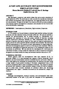
Fig. 2. The Graph GF is not error-tolerant, but is (δ = 2, r = 0.2)-error-tolerant. A proper labeling (l1 = 0, l2 = 1, l3 = 1) of GF (δ = 2, r = 0.2) is a solution of the VLM problem of GF . This labeling leads to a haplotype pair Hl = 0 1 1 / 1 0 0 which is also optimal under the MEC criterion.

has not been visited before, mark vj visited, enqueue vj into Q, set C[j] = s, and finally label vj according to the weights n0 and n1 of ei,j : if n0 > n1 , label vj with the same label of vi , that is, lj = li ; otherwise, label vj with the label different from li , that is, lj = 1−li . Once Q is empty, the procedure returns true, indicating that the connected component starting from vs is (δ, r)error tolerant and that l is its proper labeling. The connected component starting from vs may not be (δ, r)-error tolerant. In this case, we raise the thresholds by adding 1 to δ and 0.1 to r and call the procedure BFS-Labeling again with the starting vertex vs . In this way the procedure BFS-Labeling is repeatedly called until it returns true. When r becomes larger than 1, BFS-Labeling will certainly return true. Therefore, the procedure BFS-Labeling is called at most 10 times for each vertex. After the (δ, r)-error tolerant component that starts from vs is found, we exclude all its vertices from further search for error-tolerant components (i.e., virtually remove all its vertices from GF ). To find the next error-tolerant component (if any), we choose a vertex that has not yet been visited as the new starting vertex vs , reset (δ, r) to (δ0 , r0 ), and then call the procedure BFS-Labeling. The entire procedure above is implemented in Vertex-Labeling (see Appendix C). 2.2.2

Correcting sequencing errors.

The above procedure partitions GF into a number of error-tolerant components with respect to different (δ, r). There may exist many edges that connect different components, each of which is invalid with respect to a specific (δ, r). However, the haplotype information already phased on the SNP loci corresponding to an error-tolerant component could help to detect and correct some sequencing errors in the fragments, which in turn may change the weights of edges connecting different components and make them valid. Given a fragment f that spans two or more errortolerant components, we detect sequencing errors as follows. Suppose that f covers at least three SNP loci si1 , . . . , sik within an error-tolerant component

s1

s2

.

0

0

. .

e2,4

(n0, n1) = (0, 4) 1

1

... ... ...

.

e1,3

s4

... ...

.

fi

s3

l1 = 0 v1

e1,2 (1, 3)

l2 = 1 v2

(1, 1) e2,3

(2, 3)

l3 = 1 v3

e3,4 (1, 1)

v4

e1,4 (0, 1)

F

GF Error correction

s1

s2

.

. . .

0

1

F

e2,4

(n0, n1) = (0, 4) 1

... ... ...

e1,3

s4

... ...

.

fi

s3

1

l1 = 0 v1

e1,2 (0, 4)

l2 = 1 v2

(2, 0) e2,3

(3, 2)

l3 = 1 v3

e3,4 (1, 1)

v4

e1,4 (0, 1)

GF

Fig. 3. A sequencing error is detected by comparing the fragment and the labels of an error-tolerant component.

C. Let the sequence of the labels of vertices in C corresponding to si1 , . . . , sik be li1 , . . . , lik . If the Hamming distance between f [i1 ], . . . , f [ik ] and li1 , . . . , lik is smaller than k/2, every entry f [it ] not equal to lit is regarded as a sequencing error; otherwise, if the Hamming distance is greater than k/2, every entry f [it ] equal to lit is regarded as a sequencing error. For each sequencing error f [it ] detected, we flip it (i.e., f [it ] = 1−f [it ]) and then adjust the weights of affected edges in GF accordingly. For example, in Figure 3, the second allele of the fragment ”0 0 1 1” can be regarded as a sequencing error by comparing it with the labels l1 = 0, l2 = 1 and l3 = 1 of the error-tolerant component. After this error is corrected in the fragment, the weights of e1,2 , e2,3 , and e2,4 are adjusted to (0, 4), (3, 2), and (2, 0), respectively. Combining error-tolerant components. To do so, we contract each error-tolerant component into a single vertex and then iterate the procedure

JOURNAL OF LATEX CLASS FILES, VOL. 6, NO. 1, JANUARY 2014

(1, 2) l1 = 0 v1

l2 = 1 v2

l3 = 1 v3

(0, 1)

v4

Contraction (n0, n1) = (1, 0) + (2, 1) = (3, 1) l1 = 0 v1

l2 = 1 v2

l3 = 1 v3

v4

6

from a vertex vs and obtain a linear sequence of the components in their order of being visited. Taking the first three components from the sequence, we consider all four possible ways to combine them and choose the one that gives the least sum weight of incompatible edges. After these three components are combined into one, we continue with the first three components in the new sequence, until all components are combined together. The pseudocode of the algorithm Linkage Graph Haplotyping (LGH) is given in Appendix A, and is further illustrated in Figure 5.

Fig. 4. Component contraction.

3 Vertex-Labeling on the resulting condensed linkage graph. Let Bi denote the error-tolerant component to which vi belongs. As vC[i] is the starting vertex of Bi , lC[i] is always 0. Thus, vC[i] is called the root of Bi and used to represent Bi . For an edge e = (vi , vj ) within an error-tolerant component, we simply remove it from the graph GF . For an edge e = (vi , vj ) across two different components, we remove it from GF after adding its weights to the edge e0 = (vC[i] , vC[j] ) as follows: since lC[i] = lC[j] = 0, if li = lj , we add e.n0 to e0 .n0 and e.n1 to e0 .n1 ; otherwise we add e.n0 to e0 .n1 and e.n1 to e0 .n0 (see Appendix D). At the ˜F end, we would obtain a condensed linkage graph G with only edges between the roots of error-tolerant components (see Figure 4 for a simple illustration). Then we reset those roots unvisited and invoke ˜ F to find errorthe procedure Vertex-Labeling on G tolerant components as we did earlier. If the roots of two or more error-tolerant components of GF are ˜ F , then found in a same error-tolerant component of G we combine them into one and update the labels of their vertices as follows. For every vertex vit rather than a root (i.e., it 6= C[it ]), we flip lit if and only if ˜F , lC[it ] was flipped in the condensed linkage graph G and finally reset C[it ] = C[C[it ]]. The above procedure iterates until no components could be combined further. When the above iteration stops, there may still exist more than one component. In most cases, the edges across these components are invalid even with respect to the initial threshold (δ0 , r0 ), and thus it is errorprone to combine these components together. For the sake of high haplotyping accuracy, we recommend to output a block of haplotype pair for each component. To obtain long haplotype blocks, it is preferable to sequence more fragments across neighboring components. In case a complete haplotype pair is desired for a two-locus linkage graph GF , we combine the components into one as follows. Since GF is connected, ˜ F last seen from the the condensed linkage graph G above iteration procedure is also connected with only the roots of the components. After marking all the ˜ F unvisited, we start a depth-first search vertices of G

R ESULTS

Previous studies showed that HapCut, ReFHap and H-BOP are among the fastest and most accurate heuristic algorithms [7], [11], [17], [18]. Recently, two Bayesian inference based algorithms MixSIH [29] and HapTree [30] were also introduced. We thus compare our algorithm with these five state-of-the-art algorithms in this study. The C source code of the newest version v0.7 of HapCut (updated on Mar 26, 2014), the C++ source code of MixSIH and the Python program HapTree (v1.0) were downloaded from http: //sites.google.com/site/vibansal/software/hapcut, http://sites.google.com/site/hmatsu1226/software/ mixsih and http://groups.csail.mit.edu/cb/haptree, respectively. As both ReFHap and H-BOP were implemented in the Java package SIH, we also implemented LGH in Java and embedded it in SIH. LGH has a parameter combine-into-one. If combineinto-one is true, LGH is forced to reconstruct a single haplotype block for each connected component of GF . Otherwise, multiple haplotype blocks may be returned without combining them into one. To ensure that our algorithm returns the same number of haplotyping blocks as other tested algorithms, we run LGH with the parameter setting combine-into-one = true (denoted as LGHc). All the tests below are conducted on a Linux 64 bit PC with 2.5GHz CPU and 4GB RAM. When the underlying real haplotype pair is known, the number of switch errors (SEs) is commonly used to measure the haplotyping accuracy. Let (h0 , h1 ) be a haplotype pair reconstructed by an algorithm and (h∗0 , h∗1 ) be the real haplotype pair. Let (s1 , ..., sk ) be the ordered sequence of SNP loci with alleles phased in (h0 , h1 ). We say a switch error occurs between si and si+1 , where 1 ≤ i < k, if one of h0 [si , si+1 ]/h1 [si , si+1 ] and h∗0 [si , si+1 ]/h∗1 [si , si+1 ] is “0 0 / 1 1”, but the other is “0 1 / 1 0”. However, comparison of the number of switch errors is biased against the reconstructed haplotype pairs which are longer in the phased length (i.e., the number of SNP loci where the alleles are determined in the haplotype pair). For example, the haplotype pair “0 - 0 / 1 - 1” has no SE but “0 0 0 / 1 1 1” has 2 SEs when the real haplotype pair is “0 1 0 /

JOURNAL OF LATEX CLASS FILES, VOL. 6, NO. 1, JANUARY 2014

s1

s2

s3

s4

s5

s6

f1 1 f2 1 f3 1 f4 0 f5 0 f6 f7 f8 f9 f10 f11 -

0 0 1 0 1 0 -

0 0 1 1 0 1 -

1 1 0 1 0 1

0 1 0 1 1

1

7

(1, 0)

(n0, n1) = (0, 4)

l6 = ? l5 = ? l3 = ? l4 = ? l2 = ? v2 v3 v4 v5 v (1, 3) (1, 3) (2, 3) (1, 0) 6 (1, 1) C[1] = 1 C[2] = 2 C[3] = 3 C[4] = 4 C[5] = 5 C[6] = 6 l1 = ? v1

(0, 1)

(1, 1)

(1, 0)

(n0, n1) = (0, 4)

l6 = ? l5 = ? l3 = 1 l4 = ? l2 = 1 v2 v3 v4 v5 v (1, 3) (1, 1) (1, 3) (2, 3) (1, 0) 6 C[1] = 1 C[2] = 1 C[3] = 1 C[4] = 4 C[5] = 5 C[6] = 6 l1 = 0 v1

(0, 1)

(1, 1)

(1, 0)

(0, 1)

(n0, n1) = (0, 4)

l6 = 0 l5 = 1 l3 = 1 l4 = 0 l2 = 1 v2 v3 v4 v5 v (1, 3) (1, 3) (2, 3) (1, 0) 6 (1, 1) C[1] = 1 C[2] = 1 C[3] = 1 C[4] = 4 C[5] = 4 C[6] = 6 l1 = 0 v1

(0, 1)

(1, 1)

(1, 0)

(c) ( ’ r' = (1, 0.1)

(a) Fragments F (n0, n1) = (0, 4)

(1, 0)

(b) ( r = (1, 0.1)

l6 = 0 l5 = 1 l3 = 1 l4 = 0 l2 = 1 v2 v3 v4 v5 v (1, 3) (1, 1) (1, 3) (2, 3) (1, 0) 6 C[1] = 1 C[2] = 1 C[3] = 1 C[4] = 4 C[5] = 4 C[6] = 6 l1 = 0 v1

(0, 1)

(1, 1)

(1, 0)

(d) ( ’ r' = (2, 0.2)

(1, 0)

(e) f5 “001-0-” is corrected into “011-0-”

(1, 1) + (0, 1) + (1, 1) + (0, 1)

(2, 4) (0, 1)

l1 = 0 v1 C[1] = 1

l2 = 1 v2 C[2] = 1

l3 = 1 v3

(1, 1)

C[3] = 1

l4 = 0 v4 C[4] = 4

l5 = 1 v5

v (1, 0) 6 C[5] = 4 C[6] = 6

(0, 1)

(1, 1)

l6 = 0

l1 = 0 v1 C[1] = 1

l2 = 1 v2 C[2] = 1

l2 = 1 v2

l3 = 1 v3

l4 = 1 v4

C[1] = 1

C[2] = 1

C[3] = 1

C[4] = 1

Block #1

(h) ( ’ r' = (1, 0.1)

C[3] = 1

l4 = 1 v4 C[4] = 1

l5 = 1 v5

l6 = 0 v6

C[5] = 4 C[6] = 6 (1, 1)

(1, 0) + (0, 1)

(g) ( ’ r' = (1, 0.1)

(f) ( ’ r' = (2, 0.2)

l1 = 0 v1

l3 = 1 v3

l5 = 0 v5

l6 = 0

C[5] = 1 (1, 1)

C[6] = 6

v6

l1 = 0 v1

l2 = 1 v2

l3 = 1 v3

l4 = 1 v4

C[1] = 1

C[2] = 1

C[3] = 1

C[4] = 1

l5 = 0 v5

l6 = 0

C[5] = 1

C[6] = 1

v6

Block #2

(i) ( ’ r' = (1, 0.1)

Fig. 5. An illustration of Algorithm LGH with (δ, r) = (1, 0.1). Dashed lines denote invalid edges with respect to (δ 0 , r0 ). (a) The input fragments F . (b) The two-locus linkage graph G of F that is constructed at Step 1. (c) In a breadth-first search starting from v1 , the edge e2,3 is not compatible with the labels of v2 and v3 , therefore G is not (δ 0 = 1, r0 = 0.1)-error tolerant. BFS-Labeling(G, s = 1, δ 0 , r0 ) called by Vertex-Labeling at Step 2 returns false. (d) At Step 2, Vertex-Labeling increases (δ 0 , r0 ) to (2, 0.2) and call BFS-Labeling(G, 1, δ 0 , r0 ), BFS-Labeling(G, 4, δ 0 , r0 ) and BFS-Labeling(G, 6, δ 0 , r0 ), all of which return true. Thereafter, the vertices of G have been partitioned into three components and properly labeled by Vertex-Labeling. (e) At Step 4, the third allele of the fragment f5 is detected as a sequencing error and corrected, and the related weights of e3,5 are adjusted accordingly. (f) At Step 5, all edges whose adjacent vertices are in same components are removed, and the edges between different components are merged so that there are only edges between the roots of components. (g) (δ 0 , r0 ) is restored to (1, 0.1), and Vertex-Labeling is called again to connect two components with roots v1 and v4 , and the label of v4 will be flipped to 1. (h) In the case that combine-into-one is false, two components are left with roots v1 and v6 respectively. And at Step 7, since lC[5] (i.e., l4 ) has been changed from 0 to 1, l5 should be flipped from 1 to 0. At the end, the algorithm output two blocks of haplotype pair: 01110/10001 for SNP loci {s1 , s2 , s3 , s4 , s5 } and 0/1 for SNP locus s6 . (i) In the case that combine-into-one is true, the two components will be combined into one at Step 6, in which C[6] will be changed to 1, and l6 remains unchanged. A complete haplotype pair 011100/100011 is output at Step 7.

JOURNAL OF LATEX CLASS FILES, VOL. 6, NO. 1, JANUARY 2014

1 0 1”. To correct for bias, we compute the expected number of switch errors of a haplotype pair when the ‘holes’ are filled with “0/1” or “1/0” randomly, where holes refer to those loci with unphased alleles. We call this expected number of switch errors the number of adjusted SEs, and use it to assess the haplotype reconstruction accuracy. When the underlying real haplotype pair is unknown, the number of corrected errors (CEs) is often used as a performance metric. For a, b ∈ {0, 1, −}, define d(a, b) = 1 if a, b 6= − and a 6= b; otherwise, d(a, b) = 0. Given a set of fragments F and a haplotype pair H =P (h1 , h2 ) on loci (s1 , ..., Psn ). We define d(H, f ) = min( i=1,...,n d(h1 [i], f [i]), i=1,...,n d(h2 [i], f [i])) for each fragment f of F . If H is the underlying real haplotype pair, there will be at least CEs(H, F ) sequencing errors in F , where P CEs(H, F ) = f ∈F d(H, f ). As in the case of SEs, comparison of the number of CEs also favors the haplotype pairs with many unphased loci. Therefore, we compute the expected number of CEs when the holes in H are filled with “0/1” or “1/0” randomly. This expected number is analogously called the number of adjusted CEs. A SIH algorithm usually returns a number of haplotype blocks rather than a single haplotype pair as output. It is so especially when GF is not connected. Therefore, we use the number of reconstructed haplotype blocks to measure the reconstruction integrity of a SIH algorithm. Moreover, (adjusted) switch errors as well as (adjusted) corrected errors are summed over all the reconstructed haplotype blocks. 3.1

Simulation Results

We use two different methods to generate simulation datasets for performance evaluation. All the reported results are averaged over 100 repeated experiments. The first method was previously described in [17], and its main advantage is that we can control the average number of SNPs that a fragment covers. It first randomly generates a haplotype h1 of n SNPs and let the other haplotype h2 be the bit-wise complement of h1 . Then, m fragments are randomly sampled with equal probability from either haplotype such that their lengths follow a normal distribution with mean l and variance 1. Finally, every allele of fragments is flipped with probability e or substituted by ‘−’ with probability g except at the two ends of the fragments to introduce sequencing errors and gaps. We fix the haplotype length n = 100 (i.e. 100 heterozygous SNPs) and the gap rate g = 0.1. The (fragment) coverage c refers to the average number of allele calls at a SNP locus. We generate different simulated fragment datasets by varying the sequencing error rate e, the average fragment length l, and the total number of fragments m.

8

Figure 6 shows that the six tested algorithms are all accurate as there are less than 5 adjusted SEs in every 100 SNPs of a reconstructed haplotype pair. Especially when l ≥ 4, c ≥ 6 and e < 0.05, a high-quality haplotype pair can be reconstructed by the algorithms with e.n1 and lj == li then continue; if e.n0 ≤ e.n1 and lj 6= li then continue; for each vi ∈ V do { visited[i] = false; C[i] = i; } return false; } } } //end of for vi = Q.DeQueue(); } //end of while return true; }

A PPENDIX C P ROCEDURE V ERTEX -L ABELING Vertex-Labeling(G, δ, r) //The procedure returns the number of connected components //that are (δ 0 , r 0 ) error-tolerant with δ 0 ≥ δ and r 0 ≥ r. { n = the number of vertices of G; #blocks = 0; for i = 1, ..., n do { δ 0 = δ; r 0 = r; if not visited[i] then { while BFS-Labeling(G, i, δ 0 , r 0 ) == false do { δ 0 = δ 0 + 1; r 0 = r 0 + 0.1; } #blocks++; } } return #blocks; }

A PPENDIX D P ROCEDURE C OMPONENT-C ONTRACTING Component-Contracting(G) { for each edge e = (vi , vj ) of G do if C[i] == C[j] then remove e from G; else { e0 = (vC[i] , vC[j] ); if e0 is not e then { if li == lj then { e0 .n0 = e0 .n0 + e.n0 ; e0 .n1 = e0 .n1 + e.n1 ; } else {e0 .n0 = e0 .n0 + e.n1 ; e0 .n1 = e0 .n1 + e.n0 ;} remove e from G; } } for each vertex vi of G do { if C[i] == i then visited[i] = false; } }

ACKNOWLEDGMENTS This research is supported in part by Singapore Ministry of Education Academic Research Fund (MOE2012-T2-1-055) and the National Natural Science Foundation of China under grant NO. 61370172 and NO. 61232001.

JOURNAL OF LATEX CLASS FILES, VOL. 6, NO. 1, JANUARY 2014

12

TABLE 4 The summary statistics of the real datasets. NA12878 MP1 HuRef

#Heterozygous SNPs 1,704,166 2,137,482 1,966,696

#Fragments 285,341 1,165,988 3,875,104

Average fragment length 18.03 17.40 3.21

Average fragment coverage 3.02 9.50 6.32

TABLE 5 The test results on the NA12878 dataset. Adjusted SEs Adjusted SEs per 100 loci Adjusted CEs Adjusted CEs per 100 calls Number of phased SNPs Phased block length N50 (SNPs) Running time (seconds)

ReFHap 35,569.5 2.09 116,173 2.26 1,562,338 209 204.9

H-BOP 31,861.0 1.87 115,807 2.25 1,563,679 210 182.2

HapCut 36,503.5 2.14 199,905 3.89 1,582,652 215 15,307.3

LGHc 31,168.8 1.83 130,133 2.53 1,582,652 215 205.4

MixSIH 31,948.5 1.87 131,590 2.56 1,577,932 213 17,199.6

TABLE 6 The test results on the MP1 dataset. Adjusted CEs Adjusted CEs per 100 calls Number of phased SNPs Phased block length N50 (SNPs) Running time (seconds)

ReFHap 1,442,909.9 7.09 2,035,059 972 8,654.4

H-BOP 1,446,818.8 7.11 2,038,297 974 2,338.9

HapCut 1,862,905.3 9.16 2,066,685 1010 68,052.0

LGHc 1,524,609.2 7.49 2,066,685 1010 1,587.4

MixSIH 1501372.0 7.40 2,060,549 1004 157,971.5

TABLE 7 The test results on the HuRef dataset. Adjusted CEs Adjusted CEs per 100 calls Number of phased SNPs Phased block length N50 Running time (seconds)

ReFHap 238,892.6 1.92 1,776,175 370 85,102.5

H-BOP 237,008.1 1.91 1,777,903 370 357.0

R EFERENCES

[8]

[1]

[9]

[2]

[3] [4] [5] [6] [7]

S. Levy, G. Sutton, P. C. Ng, L. Feuk, A. L. Halpern, B. P. Walenz, N. Axelrod, J. Huang, E. F. Kirkness, G. Denisov, Y. Lin, J. R. MacDonald, A. W. C. Pang, M. Shago, T. B. Stockwell, A. Tsiamouri, V. Bafna, V. Bansal, S. A. Kravitz, D. A. Busam, K. Y. Beeson, T. C. McIntosh, K. A. Remington, J. F. Abril, J. Gill, J. Borman, Y. H. Rogers, M. E. Frazier, S. W. Scherer, R. L. Strausberg, and J. C. Venter, “The diploid genome sequence of an individual human,” PLoS Biology, vol. 5, no. 10, pp. e254–e254, 2007. E. F. Kirkness, R. V. Grindberg, J. Yee-Greenbaum, C. R. Marshall, S. W. Scherer, R. S. Lasken, and J. C. Venter, “Sequencing of isolated sperm cells for direct haplotyping of a human genome,” Genome Res, vol. 23, no. 5, pp. 826–32, 2013. H. Yang, X. Chen, and W. H. Wong, “Completely phased genome sequencing through chromosome sorting,” Proc Natl Acad Sci U S A, vol. 108, no. 1, pp. 12–7, 2011. The 1000 Genomes Project Consortium, “A map of human genome variation from population-scale sequencing,” Nature, vol. 467, no. 7319, pp. 1061–73, 2010. R. Tewhey, V. Bansal, A. Torkamani, E. J. Topol, and N. J. Schork, “The importance of phase information for human genomics,” Nat Rev Genet, vol. 12, no. 3, pp. 215–23, 2011. J. P. Casey et al., “A novel approach of homozygous haplotype sharing identifies candidate genes in autism spectrum disorder,” Hum Genet, vol. 131, no. 4, pp. 565–79, 2012. V. Bansal and V. Bafna, “HapCut: an efficient and accurate algorithm for the haplotype assembly problem,” Bioinformatics, vol. 24, no. 16, pp. i153–9, 2008.

[10] [11]

[12] [13] [14]

[15]

[16]

HapCut 244,851.3 1.97 1,789,147 374 16,014.5

LGHc 251,913.8 2.03 1,789,147 374 248.0

MixSIH 424,963.0 3.42 1,788,766 374 202,020.8

S. R. Browning and B. L. Browning, “Haplotype phasing: existing methods and new developments,” Nat Rev Genet, vol. 12, no. 10, pp. 703–14, 2011. M. Xie, J. Wang, J. Chen, J. Wu, and X. Liu, “Computational models and algorithms for the single individual haplotyping problem,” Current Bioinformatics, vol. 5, no. 1, pp. 18–28, 2010. X. S. Zhang, R. S. Wang, L. Y. Wu, and L. Chen, “Models and algorithms for haplotyping problem,” Current Bioinformatics, vol. 1, no. 1, pp. 105–114, 2006. J. Duitama et al., “Fosmid-based whole genome haplotyping of a hapmap trio child: evaluation of single individual haplotyping techniques,” Nucleic Acids Res, vol. 40, no. 5, pp. 2041–53, 2012. J. O. Kitzman et al., “Haplotype-resolved genome sequencing of a Gujarati Indian individual,” Nat Biotechnol, vol. 29, no. 1, pp. 59–63, 2011. E. K. Suk et al., “A comprehensively molecular haplotyperesolved genome of a European individual,” Genome Res, vol. 21, no. 10, pp. 1672–85, 2011. V. Kuleshov, D. Xie, R. Chen, D. Pushkarev, Z. Ma, T. Blauwkamp, M. Kertesz, and M. Snyder, “Whole-genome haplotyping using long reads and statistical methods,” Nat Biotechnol, vol. 32, no. 3, pp. 261–6, 2014. G. Lancia, V. Bafna, S. Istrail, R. Lippert, and R. Schwartz, “SNPs problems, complexity and algorithms,” in Proc. Ann. European Symp. on Algorithms (ESA), ser. Lecture Notes in Computer Science, F. M. auf der Heide, Ed., vol. 2161. Berlin/Heidelberg: Springer, August 2001, pp. 182–193. R. Lippert, R. Schwartz, G.Lancia, and S. Istrail, “Algorithmic strategies for the single nucleotide polymorphism haplotype assembly problem,” Brief. Bioinform, vol. 3, no. 1, pp. 1–9, 2002.

JOURNAL OF LATEX CLASS FILES, VOL. 6, NO. 1, JANUARY 2014

[17] J. Duitama, T. Huebsch, G. McEwen, E.-K. Suk, and M. R. Hoehe, “ReFHap: a reliable and fast algorithm for single individual haplotyping,” in Proceedings of the First ACM international Conference on Bioinformatics and Computational Biology. Niagara Falls, New York: ACM, August 02-04 2010, pp. 160– 169. [18] M. Xie, J. Wang, and T. Jiang, “A fast and accurate algorithm for single individual haplotyping,” BMC Systems Biology, vol. 6, no. Suppl 2, p. S8, 2012. [19] R. S. Wang, L. Y. Wu, Z. P. Li, and X. S. Zhang, “Haplotype reconstruction from snp fragments by minimum error correction,” Bioinformatics, vol. 21, no. 10, pp. 2456–2462, 2005. [20] M. Xie, J. Wang, and J. Chen, “A model of higher accuracy for the individual haplotyping problem based on weighted SNP fragments and genotype with errors,” Bioinformatics, vol. 24, no. 13, pp. i105–13, 2008. [21] D. He and E. Eskin, “Hap-seqX: expedite algorithm for haplotype phasing with imputation using sequence data,” Gene, vol. 518, no. 1, pp. 2–6, 2013. [22] W. Y. Yang, F. Hormozdiari, Z. Wang, D. He, B. Pasaniuc, and E. Eskin, “Leveraging multi-SNP reads from sequencing data for haplotype inference,” Bioinformatics, 2013. [23] M. Xie, J. Chen, and J. Wang, “Research on parameterized algorithms of the individual haplotyping problem.” J Bioinform Comput Biol, vol. 5, no. 3, pp. 795–816, 2007. [24] M. Xie, J. Wang, and J. Chen, “A practical parameterised algorithm for the individual haplotyping problem mlf,” Mathematical Structures in Computer Science, vol. 20, no. 5, pp. 851– 863, 2010. [25] D. He, A. Choi, K. Pipatsrisawat, A. Darwiche, and E. Eskin, “Optimal algorithms for haplotype assembly from wholegenome sequence data,” Bioinformatics, vol. 26, no. 12, pp. i183–90, Jun 15 2010. [26] Z. Z. Chen, F. Deng, and L. Wang, “Exact algorithms for haplotype assembly from whole-genome sequence data,” Bioinformatics, vol. 29, no. 16, pp. 1938–45, 2013. [27] L. M. Genovese, F. Geraci, and M. Pellegrini, “SpeedHap: an accurate heuristic for the single individual snp haplotyping problem with many gaps, high reading error rate and low coverage,” IEEE/ACM Trans Comput Biol Bioinform, vol. 5, no. 4, pp. 492–502, 2008. [28] F. Deng, W. Cui, and L. Wang, “A highly accurate heuristic algorithm for the haplotype assembly problem,” BMC Genomics, vol. 14 Suppl 2, p. S2, 2013. [29] H. Matsumoto and H. Kiryu, “MixSIH: a mixture model for single individual haplotyping,” BMC Genomics, vol. 14 Suppl 2, p. S5, 2013. [30] E. Berger, D. Yorukoglu, J. Peng, and B. Berger, “HapTree: a novel Bayesian framework for single individual polyplotyping using NGS data,” PLoS Comput Biol, vol. 10, no. 3, p. e1003502, 2014. [31] D. C. Richter, F. Ott, A. F. Auch, R. Schmid, and D. H. Huson, “MetaSim: a sequencing simulator for genomics and metagenomics,” PLoS One, vol. 3, no. 10, p. e3373, 2008. [32] The 1000 Genomes Project Consortium, “An integrated map of genetic variation from 1,092 human genomes,” Nature, vol. 491, no. 7422, pp. 56–65, 2012.

13

Minzhu Xie received his MEng and PhD degrees in computer science from Central South University, China, in 2003 and 2008, respectively. He is a professor in College of Physics and Information Science, Hunan Normal University, China. His current research interest is bioinformatics.

Jianxin Wang received his BEng and MEng degrees in computer engineering from Central South University, China, in 1992 and 1996, respectively, and the PhD degree in computer science from Central South University, China, in 2001. He is the vice dean and a professor in School of Information Science and Engineering, Central South University, China. His current research interests include algorithm analysis and optimization, parameterized algorithm, bioinformatics, and computer network. He has published more than 150 papers in various international journals and refereed conferences. He is a senior member of the IEEE.

Xin Chen received his PhD degree from Peking University, Beijing, China, in 2001. Currently, he is an assistant professor in the Division of Mathematical Sciences, School of Physical and Mathematical Sciences, Nanyang Technological University, Singapore. His research interests include computational biology and bioinformatics, algorithms, and data compression.