International Journal of Security and Its Applications Vol. 3, No. 3, July, 2009
Lightweight Anomaly Detection System with HMM Resource Modeling 1
1
Midori Sugaya, 2Yuki Ohno, and 2Tatsuo Nakajima
Dependable Embedded OS R&D Center, Japan Science and Technology Agency, Tokyo, Japan 2 School of Science and Engineering, Waseda University, Tokyo, Japan 1
[email protected], 2{yuuki-ohno,tatsuog}@dcl.info.waseda.ac.jp Abstract
In this paper, a lightweight anomaly detection infrastructure named Anomaly Detection by Resource Monitoring is presented for Information Appliances. We call it Ayaka for short. It provides a monitoring function for detecting anomalies, especially attacks which are a symptom of resource abuse, by using the resource patterns of each process. Ayaka takes a completely application black-box approach, based on machine learning methods. It uses the clustering method to quantize the resource usage vector data and then learn the normal patterns with a hidden Markov Model. In the running phase, Ayaka finds anomalies by comparing the application resource usage with the learned model. This reduces the general overhead of the analyzer and makes it possible to monitor the process in real-time. The evaluation experiment indicates that our prototype system is able to detect anomalies such as SQL injection and buffer overrun with a minimum of false positives and small (about 1%) system overhead, without previously defined anomaly models. Keywords: anomaly detection, security, operating system, system resource, HMM, model
1. Introduction Current information appliances, such as cell-phones, car navigation systems, home appliance servers, and PDAs, currently have greatly extended computing environments to connect to the Internet. However, in contrast to the personal computer, information appliances still lack the underlying support for accessing an open network. Generally, users of such appliances do not have professional skills and knowledge about the threats of an open network, and without filtering of the routers in their gateways, these systems are an easy target for attacks. For example, in 2004 a hard disk recorder that was connected to the Internet without any safeguards was attacked and misused by hackers for massive spamming around the world [19]. To detect these problems before the damage expands, detection systems are configured with a number of signatures that support the detection of attacks. Numerous approaches have been presented in this area. Surveys of implemented intrusion detection systems, many of which are already in operation, can be found in several practical systems such as Solaris [29], Windows [1], and Linux [23]. In the research area, several effective techniques for detecting intrusions have been developed. There are statistical, rule-based approaches [13]; Neural Networks [5]; and Generic Algorithms [24]. However, most research assumes mission critical servers and personal computers. The requirements for information appliances are rather different, from the point of limited resources, from those of information appliances. Therefore,
35
International Journal of Security and Its Applications Vol. 3, No. 3, July, 2009
we need to consider small overhead, from the point of view of both time and space. Second, there is a need to support diverse applications that are implemented with a variety of programming languages and different kinds of hardware. Mission critical servers do not care about such diversities, since most servers run similar applications and hardware [2, 9, 8]. Third, we need to consider a method for unknown anomaly detection in online systems. In information appliances, we need to assume a variety of architectures and programming languages. In that situation, not only intrusion detection, but also attacks or misuse, must be pre-supposed. The general meaning of anomaly detection is important for this area. For detecting an unknown anomaly, real-time detection is also important. Non real-time static analysis or debugging should not be expected for information appliances as a background service, since their resources are limited. Static analysis may consume a considerable amount of CPU time, expensive detection algorithms should be delegated to faster servers in wide area networks. In this paper, we focus on a lightweight online anomaly detection system that is used for information appliances. We propose Ayaka, a new system that monitors processes for resource usage and detects anomalies without special knowledge of the underlying system. The contribution of this paper is to present a method that uses resource usage (CPU, memory, and network resources) of specific processes with an adaptable sampling period, and models the normal behavior of the process with a learning method to detect unknown anomalies online. This method can generally be applied to embedded systems because there are no dependencies on programming languages, platform, or architecture. The nature of this approach should bring great benefits for developing new embedded products without the modification of applications and tuning anomaly models that depend on the platforms. Moreover, our approach is blessed with low overhead. To achieve this, we use the clustering method for analyzing the behavior of processes and storing just the precision rate of models. This can effectively reduce the overhead at runtime detection, since it just compares the rate of the models via online analysis without loss of effectiveness and thus keeps a precise detecting rate. We will show the effectiveness of this approach in our evaluation. The remainder of this paper describes our approach to automating problem detection for processes by analyzing resource usage. Section 2 presents related work. Section 3 describes the approach and algorithm of our methodology. Section 4 shows the implementation of the system. Section 5 describes our experimental validation, Section 6 presets further discussion of important issues for our approach, and finally, we conclude our paper in Section 7.
2. Related Work In previous work, Koral describes the objective of anomaly detection. He said it is to establish usage patterns within user audit trails over a duration of time, and use these usage patterns as profiles of ”normal” system activity[18]. The objective of anomaly detection is not different these days, but varieties of approaches are available to analyze data for finding anomalies. Stefan [27] classified anomaly detection into two types. One is programmed and the other is self-learning. The programmed (signature) approach requires someone to detect certain anomalous events, and self-learning systems learn by example what constitutes normal for the installation. Programmed (signature) data bases are all of the type that makes signature decisions on anomaly data. One could detect anomalies from signature data. The common research paradigm in the programmed and signature data base approach is the expert system which codes knowledge about attacks as if-then implication rules or descriptive statistics. It builds a profile of normal statistical behavior by various parameters of the system, and collects descriptive statistics on a number of those parameters. The known statistical
36
International Journal of Security and Its Applications Vol. 3, No. 3, July, 2009
profile-based Intrusion Detection Expert System (IDES) is presented in [3]. IDES processes each new audit record as it enters the system, and verifies it against the known profile for both the subject, and the group of the subject, should it belong to one. IDES also verifies each session against known profiles when the session is completed. Ilgun [17] uses state transition to model and detect abnormal transitions from the audit trail file. Kumar [21, 26] employs colored Petri-nets for signature based intrusion detection. These approaches gain the merit of modeling the pattern of the anomaly. Several projects on security [15, 13] also take these signature-based approaches. In these signature approaches, there are several limitations. First, finding sporadic user environments and establishing profiles of normal user behavior would be difficult [18]. This leads to a potentially large number of false positives. Second, it is difficult to efficiently specify an order in which to match facts within the natural framework of expert system shells. Third, including software engineering concerns with the maintenance of the knowledge base and the quality of the rules points out they can only be as good as the human devising them [21]. Fourth, the signature based approach provides high precision for the detection rate. However, these approaches tend to increase the overhead to take more detailed logs of the audit trails. Self-learning is the other kind of approach for anomaly detection. It focus on a model that builds a normal model of audit data (or data containing no intrusions) and detects intrusions based on detecting deviations from the normal model[12]. This approach finds unknown anomalies. Some of the earliest work on self-learning is commonly considered to be those reported by Anderson [4] and Denning [6]. They provide a detection system that studies historic audit data to produce rules describing “normal” behavior. The rules are fed to an expert system that evaluates recent audit data for violations of the rules, and alerts the system when the rules indicate anomalous behavior. In terms of those rules, this method identifies computer transactions that are at variance with historically established usage patterns. The authors consider a figure of around 500-1,000 audit. These descriptive statistic approaches are also taken in IDES projects [3], and EMERALD [25]. Considering time series data, Hyperview [14] provides the untested approach of mapping the time series to the inputs of a neural network. At the time, the usual approach was to map inputs to a window of time series data, shifting the window by one between evaluations of the network. System call traces for a self-learning approach are a common type of audit data collected for performing IDS (Intrusion Detection System) processes. A system call trace is the ordered sequence of system calls that a process performs during its execution. Steven [16] presents an approach to collect a sequence of system calls that can be the discriminator between normal and abnormal operating characteristics of several common UNIX programs by using the Hamming distance. The precision of the detection rate of Steven’s approach was relatively lower than the approaches presented by Keith [20], Eskin [12], and Warrender [30]. Keith [20] suggests function call analysis include the system calls in order not only to find anomalies, but also for use in forensic analysis. The function calls they capture are the significant events that occur in both user and kernel space. However, most of these system call/function call approaches are mainly offline since they focus on the efficiency and accuracy of the analysis, not on the computing efficiency. Moreover, the models should be different from the base operating system. This point is the difference between these approaches and our concerns. The performance of these self-learning models depends greatly on the robustness of the modeling method and the quantity and quality of the available training data. From this point, Eskin [11] presents robust methods for choosing the sliding window size and applying them to modeling system call traces. The sparse markov transducers (SMTs) algorithm can reduce the time of calculation [12]. The results show that method suitable if they tune it, so that the false positives decrease relatively. However, the
37
International Journal of Security and Its Applications Vol. 3, No. 3, July, 2009
nature of the system call requires the availability of the sequence of logs that duplicate the function calls. It would be difficult to hide the system from the attacker.
3. Model Construction Infrastructure 3.1. Design Objectives We focus on the security issue in information appliances. To satisfy the requirements of these appliances, we will provide a lightweight anomaly detection system using a selflearning approach. To impose various requirements to make the system broadly applicable to information appliances applications, we draw on four main principles. The first is to detect unknown anomalies. To achieve the purpose, we use a machine learning technique to learn the normal behavior of the process. That makes it to possible to find the anomaly state as an inverse of the normal state, without specific knowledge of either state. The second is an application black-box approach. We model process behavior using state transactions for resource consumption and treat the application as a black-box. This approach can be generally applied to embedded system applications because it has no dependencies on programming languages and platforms. It brings development benefits for system vendors who develop new products with minimum time. The third is real-time detection. Our system provides an online processing mechanism. By using the self-learning method, it compares the learned model and the processing data profiled, and takes action accordingly that provides functions to report the result to the next higher node, or stop the process to avoid abuse of other resources. Steven [16] provides a system that finds anomalies and then follows safety procedures afterwards, our system, on the other hand, can automatically prevent extending the problem. The last principle is low overhead. To achieve real-time detection, we use a precision rate for deciding the anomalies that is calculated in the learning phase. This makes it possible to provide lightweight anomaly detection in practical use. We explain the details of all of this in the following section. 3.2. Choosing Applicable Methods 3.2.1. Requirements and Methodology The objective of Ayaka is to find anomalies, and therefore it provides functions and algorithms to do this accurately. We focus on the anomaly state transition of process resource usage that relates to non-deterministic faults and system abuse, such as DoS, fork attacks, and infinite loops that also abuse the resources. These types of anomalies have in common that they abuse the resources with some specific patterns and risk occupying system resources until the system shuts down. To present a solution for this problem, we adopted three approaches to develop our methodology.
38
Modeling the Normal Behavior of a Process: The first is modeling the normal behavior of an application to find the unknown anomaly. There is lots of research presented in related work as self-learning. We follow the basic definition, collect normal patterns, and define the model based on the patterns heuristically. At runtime, we use the models to compare the input stream with previously defined ones. In fact, there is no good solution for creating precise models that consider the runtime environment and find unknown anomalies with general versatility. We assume that a normal state of an application can be observed by the standard behavior of that application. The standard behavior is defined as
International Journal of Security and Its Applications Vol. 3, No. 3, July, 2009
some state in which there are no significant errors, or attacks, or resource abuses that come under observation. Using Resource Usage of a Process: As the second approach, we use resource information of applications. Resource usage is language-, operating system- and architecture- independent. If there are problems with applications, resource usage is surely affected. In many cases, the CPU is used for finding resource abuses in an application, but this is not enough to build a complex model of problems. To express the complex patterns of resource problems accurately, we use three resource parameters, CPU, memory, and network usage, to express a complex model of application behavior. This makes it possible to classify cases such that if an application’s CPU usage is 10%, but at the same time if the network resource usage is 0% or 90%, the models are different. Moreover, resource usage data makes possible to be independent from the operating system which system call models generally depend on. Model Learning: As the third approach, we use the machine learning technique to study the normal pattern according to domain specific information before the system works under normal operation. It is still difficult to create an exact normal pattern of an application considering the differences in its runtime environment. If there is a system that under normal operation uses 50% of its CPU resource, the anomaly might be defined as that state where 90% of the system resources are used up. But, if there is a system that uses almost 99% of its resources in normal situations, its resource usage pattern will be different and requires a high threshold to be judged as the anomaly. The essential problem is that the resource limitation totally depends on the hardware configuration of the system. Therefore, we consider ways of learning domain-specific patterns. This makes it possible to adapt to a new environment without domain specific knowledge of the system. 3.2.2. Hidden Markov Model To satisfy those requirements, we consider a way of analyzing the essential features of the resource usage model of a process. Resource usage changes continually as time goes on. We analyze this by using time series analysis methods. There are several methods used to analyze time series data. For example, Fourier analysis is one of the most famous methods used to analyze time series data. However, it needs the strong assumption that steady-state performance of the data is known, and needs to be applied to a function with an infinite period. Our resource consumption data is not usually the steady-state type. To develop effective models of applications, we need a method that can model the transitional state of resource usage. Moreover, to satisfy the last requirement, that we need to build a domain specific model of the application, we assume machine learning is needed. For these reasons, we apply the Hidden Markov Model (HMM). It is a powerful modeling technique that represents the discrete states of resource consumption of processes. This also provides the procedures for machine learning methodology. The main idea of the HMM is that an observation sequence generated by a system is represented as a finite number of states [7]. For each step, it makes a transition from its current state to another state, according to a specific probability distribution inferred from the observation symbol. It is defined by the number of states. HMM generates different models which do not have different transitional states. We use the HMM to analyze the resource data and create models of the normal state of the application with machine learning methodology. 3.2.2. Model Construction Procedure
39
International Journal of Security and Its Applications Vol. 3, No. 3, July, 2009
The procedure, starting from the resource data to developing the HMM model, is classified into the following steps. The first step is the preparation for the analysis. We cannot use the sampling data that a system generates directly as parameters for HMM, because there is too much data. Therefore, we convert the sampling data by calculating resource vectors. Then, we classify them into groups that have similarities by the clustering method. The second step is analysis of the data to create normal models of applications with HMM. To calculate the probability of the models, we use several techniques to learn the precise models of the application. We call this step model learning. The system stores the normal pattern. The third step is online analysis. According to the sampling data of the application, Ayaka evaluates whether the current state is normal or not by comparing the precision of the normal models. 3.2.4. Data Set First of all, resource consumption data from processes of an application such as CPU usage, memory usage, and network usage, is collected from the system. We define the following formula to calculate their usage. We assume a sampling period T is defined as a period. CPU resource usage Ucpu is defined as the rate of computation time C of a process within the period T. It is defined by the following formula. U cpu C / T (1) Actually, a process is both stopping and running during this period T. For example, we assume the start time of a process is Cs0 and the finish time of the process is defined as Ce0. If the process uses CPU time again, we describe the next incidence as Cs1 and Ce1. Then the general formula is defined as follows (2). U cpu i (Cei Csi ) /T (2) Memory usage is different from CPU usage at the point that it is calculated by the quantity. Memory usage Umem is defined by the rate of the quantities m consumed by each process within all the memory M that is installed in the system. As we explained in CPU usage, a process allocates and frees a memory block during a period. We assume a chunk of memory m at a time t is defined by m0 and t0, respectively. After a while, the quantity is changed to m1 at time t1, then changed to m2 at time t2. It is represented by the following formula (3).
Umem in01(ti 1 ti ) mi /T M
(3) Network usage Unet is calculated by the maximum data transfer speed v and the transferred data of the process d within the period T (4). The maximum quantity of data transfer is always changing in networks. If we define just the rate for Unet by the quantity of data transfer and the maximum quantity of data transfer within T, it will be wrong. To specify the correct rate of the traffic, we use v as a constant (1,000,000 bytes) and express the average rate of the traffic (MB/s) as the rate of the network. Unet d / v T (4) Before collecting data, we set the sampling period T to calculate resources by formulas (2) and (3). The collected data is defined as Ucpu,Umem,Unet. A set of these data is defined as a vector veci. The ith resource vector is represented as veci = (Ui,,cpu,Ui,mem,Ui,net). We make them a set and define u to represent this as a vector u = {Ucpu,Umem,Unet}. The ith collected data set is defined as ui, then the set of resources is defined as ui = {Ui,cpu,Ui,mem,Ui,net}. For example, there are two sampling data items, the ith and i + 1, the resources are described as Ui and Ui+1. The ith vector is calculated as follows. vec 1 (U 2 , cpu U 1, cpu ) 2 (U 2 , mem U 1, mem ) 2 (U 2 , net U 1, net ) 2 . The nth set of
40
International Journal of Security and Its Applications Vol. 3, No. 3, July, 2009
vectors is defined as vecn. We decide the changing point of the data is the delimiter of the data. The changing point of the boundary is u i 1 u . Using this boundary, we partition the data and apply the k-mean method. We use = 0.1 as the boundary in this paper. The advantage of computing distance between the vectors rather than the raw traces is that the tendencies of resource consumption are less sensitive to insignificant variations in application behavior. However, once an anomaly occurs, the behavior of an application changes substantially. 3.2.5. Clustering with the k-mean method Clustering is a method used to partition a data set into subsets (clusters) so that the data in each subset share a common trait. We use the proximity of similarity according to a distance measure of resource vectors. A vector consists of CPU, memory, and network resource usage Table 1. Number of Clusters (k) and Evaluation k
False negative False positive 6 0 2 14 0 4 20 0 0 False negative (Fn): The anomaly is not detected. False positive (Fp): The anomaly is reported but not present.
at a certain sampling period. In order to cluster and abstract this data, the k-mean algorithm [22] is applied with k being the number of clusters. Compared to an algorithm that creates a hierarchical tree, this one reduces the amount of calculations. The first step of the k-mean algorithm is to choose the number of clusters. The appropriate k depends on the domain. k must be determined empirically. We decided to conduct tests to find a suitable k for satisfying our results. We first evaluated the initial parameters {6, 14, 20} (shown in Table 1) as a candidate for k. The evaluation method is described in detail in Section 5.3. According to the SQL injection detection results, shown in Table 1, we found k = 20 clearly identifies the differences of anomalies more precisely than the other numbers. k-mean assigns each point to the cluster whose center (called the centroid) is the nearest. The center is the average of all the points in the cluster, which means the centroid is equal to the arithmetic mean for all dimensions. To classify the data for a cluster, we set the unique number of clusters to k and then set a parameter for the cluster as an initial centroid parameter. We define the jth cluster’s centroid as cj . At this time, the cluster that has the centroid cj is defined as Cj . The first step of the classification of the vector data ui is to select the appropriate jth cluster Cj that has the smallest distance to the point of the similarities. The nearest cluster is defined as the minimum distance between ui and centroid cj (min (|cj - uj|)). If all of the calculations of ui are finished, then, as a next step, we recomputed each centroid cj as ( u c j u ) / C j to calculate the new centroid. These steps are repeated until the convergence criterion is met. At the end, each vector ui exports the cluster number which classifies itself. For example, if the vector u1 is classified to one of the 20 clusters C3, and if u2 is classified to C1 and u3 to C2, we will see the result that the unit of emission symbols of the vectors u1, u2 and u3 are classified into C3, C1,C2. 3.3. Model Learning with HMM 3.3.1. Topology
41
International Journal of Security and Its Applications Vol. 3, No. 3, July, 2009
There are two competing HMM instances we might return to. These are the ergodic and the left-right models. In the ergodic HMM, every state of the model can be reached from every other state. Table 2 shows that the ergodic 8 is the minimum number of states and most accurate for determining false negatives and positive numbers in evaluation. In the end, we chose our model to be an ergodic HMM with 8 states, for convenience. 3.3.2. Estimating Parameters In HMM, transitions among the states are governed by a set of probabilities called transition probabilities. In a particular state, an outcome can be produced. It is only the outcome, not the state that is visible to an external observer, as states are hidden to the outside. Therefore, it is difficult to estimate the maximum likelihood. The Baum-Welch algorithm [7] estimates parameters of a given HMM and produces a new model which has a higher probability of generating the given observation sequence. This procedure is continued until no more significant improvement can be obtained. The algorithm is a general way of calculating the maximum likelihood with guaranteed convergence. In our system, an HMM Table 2. Precision compared with the Number of States and Topologies Topology left-to-right
ergodic
Num of States 6 8 10 6 8 10
False negative 1 3 3 0 0 0
False positive 1 0 0 0 0 0
model is initialized for every incoming vector and then optimized by the Baum-Welch algorithm. The Backward-forward algorithm is a method for calculating this efficiently. We use it for efficiency of the calculation. First of all, the Baum-Welch algorithm uses the forward-backward algorithm to calculate the certain probability of the ith state of time t with time series (forward) and reverse (backward). The forward probability of fi (t ) is calculated by formula (5), and the backward probability is calculated by formula (6). In this model, the transitional probability of the state i j is defined as aij, and the probability of the emission k at the time of state i is defined as bi(k). The emission of time t is defined as V(t).
fi (t ) fj (t 1) ajibi (V (t ))
(5)
j
gi (t ) aijbi (V (t 1)) gj (t 1)
(6)
j
The probability of ij which proceeds the transition i j at time of t is calculated by formula (7) at the emission sequence V ( t ) Tt 0 . In a similar way, the probability of i is calculated by formula (8) at the probability of state i at the time of t. SF shows the last state of the set under the Markov Model.
ij
fi (t ) aij bj (V (t 1) gi (t 1) k SF fk (T )
i (t ) ij (t ) j
42
(7) (8)
International Journal of Security and Its Applications Vol. 3, No. 3, July, 2009
By these calculations, the estimate aˆij of the probability of state transition aij is calculated by formula (9). The estimation of the probability value bˆj (k ) that the emission symbol is vk,
when the state is sj is calculated by formula (10). T 1
aˆij
t 0 ij (t ) T 1 t 0 i(t )
tV (t )vk j (t ) bˆj T t 0 j (t )
(9)
(10)
bi(k) is the probability that the emission is k. {V(t)} is the emission at time t. When the emission is V ( t ) Tt 0 , the probability of the data and model (precision) p is represented by the formulas shown in (5), (6), and (11). By using the Baum-Welch algorithm, HMM makes it possible to determine the model which will produce a given sequence of observations with the highest probability. It takes the sequence of observations and allocates observations to particular states based on the current values of aji and bi(k). p fi (T ) (11) i
The state transition of the process assumes it to be classified in models depending on what the process executes and the external conditions of the process in the system environment. Therefore, to improve the precision of detecting the anomaly state, we need to prepare multiple HMM for each classified model. Based on this, we arrange multiple HMM to learn each model. If the emissions are generated by HMM, we compare the symbols with the previously learned HMM. 3.3.3. Training and Detection We use precision p as the calculation result of an HMM to judge the anomaly. p is the sum of the probabilities of matching each model that is shown in formula (11). The system calculates the p at the condition of V ( t ) Tt 0 by using aji and symbol emission probability bi(k) which are learned within the training. We set a certain probability as a threshold . In the training phase, if the precision p is higher than a threshold , we decide that the input data and learned model are matched ( p ). We add the matched data to the compared model as training data. In contrast, if the values are not matched or there are no models to be matched, we create a new model and add the unmatched data to the new model as training data in the same way as in the learning process. The normal models are stored before the system starts to provide the actual services. After actual service is started, the system stores the resource usage data in particular sampling periods, and calculates vectors in the same way as in the learning process. Then, it makes clusters which are adjusted in the learning phase. Those data are eventually used to evaluate the learned model. In the operation phase, if the precision p is higher than the threshold ( p ), we decide the incoming data is normal. But if it is not ( p ), we decide it’s an anomaly.
4. Implementation 4.1. Overall architecture
43
International Journal of Security and Its Applications Vol. 3, No. 3, July, 2009
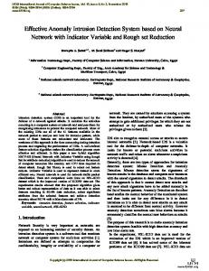
Our prototype system is developed as a kernel module on the Linux kernel 2.6.23. In Figure 1 the overall architecture of Ayaka is shown. Ayaka will start with some parameters that the administrator or system designer set. The parameters are the process IDs which need to be watched, the monitoring period, and the policy actuated when anomalies are detected. Ayaka is composed of the following three main functions.
Tracing: In Ayaka, kernel hooks are inserted to take a log of the accurate amount of resources that a process uses. Each hook traces and accumulates the amount of the resources such as CPU, memory, network resources that a process uses. The detailed hook points are described in section 4.2. To take the information from the each hook point, we use the extension of LTTng (LTT Next Generation) [10]. It provides the basic tracing facilities, such as a trace point call back mechanism, to take information from each hook in the Linux kernel. Accounting: The accounting section provides the facilities for managing the resource usage of each process or group of processes. To manage the resource consumption of processes, it provides timers and monitoring objects. If a process uses a resource such as
Figure 1. Overall Architecture
memory or a network socket, the tracing callback facilities store the information, including the amount of resources the process uses, for the monitored object. The dynamic timer manages the periodic time. When the user passes the sampling period T for Ayaka’s API, the API sets the period into the monitoring object, and the monitoring object collects the resource information of the monitored process periodically. When it reaches the next period, after calculating the utilization of the resources for each process, these statistics are stored in a ring-buffer in kernel memory that is exposed to users through /proc file systems. These accounting facilities are implemented as an extension of the Accounting System [28]. It also provides the process control functions to avoid suffering damage to resources through abuse of the process. Analysis: We implement a monitoring daemon that reads the data from the /proc file system and passes it to the analysis module, which analyzes the data. Currently, we have implemented the HMM algorithm that we described in the previous section. In learning mode, it works to learn the data to build the normal model of the process resource usage. In detection mode, by using the normal model, it can find anomalies compared with the
44
International Journal of Security and Its Applications Vol. 3, No. 3, July, 2009
trained models. At the time of detecting an anomaly, the module will report it to the accounting facilities which control the process. A process control mechanism blocks the process in a mandatory way. Generally, the module is replaceable, since a variety of methods is used according to the threat. These procedures are performed online, but it is also possible to create files from the kernel buffer that can be used for off-line analysis. 4.2. Collecting the Resource Data In this section, we describe the method used for collecting the data of a process in detail. Our tracer provides the facilities to collect the resource event and a fine-grained timestamp for the time of occurrence of the event with a timestamp counter. To collect the data for CPU, memory, and network resources, we set hooks in the following places. CPU: We set the hooks at the point of the context switch in the scheduler in order to obtain the execution time of each process accurately. Ayaka accumulates the execution time of the process for the monitoring object that the process belongs to.
Memory: We set the hooks at the point of adding PTE (Page Table Entry) and removing a page from a file page to obtain the memory consumed by each process. The same as the CPU, Ayaka accumulates the pages which a process uses in its execution. Table 3. Creates Ayaka API API create bind unbind destroy set get
Contents Creates and initializes a new monitoring object. A sampling period is needed for it. Makes a relationship to the monitoring object and a process which is monitored. Releases the process which is monitored from the host monitoring object. Destroys the memory area used by monitoring object. Makes modifications to the parameter of the monitoring object Obtains parameters from a specified monitoring object.
Network : We set the hooks at the point where a network socket buffer held and released to count the socket buffers used for the task. These hooks are available for the tracers which are loaded as a group of hooks and facilities. In our system, if a developer wants to add a new hook, it can be added by registering the hook and the callback function in it.
These hooks are available for the tracers which are loaded as a group of hooks and facilities. In our system, if a developer wants to add a new hook, it can be added by registering the hook and the callback function in it. The overhead of our tracer is less than 2.5% of the generally system overhead, however, we only use a few of the hooks that are provided by LTTng. Therefore, this reduces the general overhead of our tracer and makes monitoring as lightweight as possible. 4.3. User APIs Ayaka proposed APIs for collecting resource data in a ring-buffer in the kernel and setting the sampling period T for each process or group of processes. Ayaka’s APIs are described in Table 3. The procedures required to use our system are as follows. The developer first calls create for creating the monitoring group, which is a unit of the resource monitoring feature with the parameter of the sampling period and a certain enforcement policy. As the second step, the process ID is set to call bind to register the process ID for the monitoring group. At the time of a process bind to a monitoring group, the process or processes are under the
45
International Journal of Security and Its Applications Vol. 3, No. 3, July, 2009
control of the Ayaka monitoring system. These APIs have symmetrical APIs, such as destroy and unbind. The set and get APIs are provided for changing the parameters of the monitoring group and taking the information from the monitoring group. Our system provides a pluggable, modularized interface for the analysis of resource data. It is possible to replace the analysis method. For example, in this paper we use HMM for data analysis, but it could be easily replaced by another method without changing the core system. 4.4. Enforcement Policies Ayaka not only provides the analysis modules that detect the anomaly, but provides the enforcement functions that can control the problematic process before serious problems and critical damage arise in the system: Report the anomaly to a higher node: sends a signal to a registered process or a registered host immediately when an anomaly is detected. Block the suspicious process: blocks the process that is responsible for the anomaly in order to prevent further damage. Dump process data to another host: sends a process dump of the observed process that caused the anomaly for later analysis. These enforcement functions are available to write a policy for system calls. Ayaka provides APIs to set up the policy for the functions.
5. Experiments & Evaluation Our prototype implementation of Ayaka is based on Linux kernel modifications and augmentations. In this section, we evaluate the overhead and precision of the system. The hardware environment is an Intel(R) Pentium(R) D 2.80GHz CPU system with 2GB of memory. 5.1. Basic System Overhead To evaluate the basic overhead of Ayaka, we ran a simple calculation program on the monitoring system and measured the execution time with the CPU cycle counter (TSC counter in x86). We compare three environments. Table 4 shows the results of 1,000 executions of the program in different environments. In this table, Without Monitoring means that Ayaka is turned off. Training indicates the learning phase where Ayaka collects the data and stores the models of the normal behavior of a process. Runtime indicates that the system is working both training and detecting concurrently. In this table, we can see the overhead percentage for each environment in (B). Compared to Without Monitoring, Training increases the overhead up to 1.1% and the Runtime overhead up to 1.2%. These results show the overhead of Ayaka is small enough to use the system successfully. Table 4. System Overhead Execution Time (second) Average Execution Time Max Min (A) Ratio to Without Monitoring (B) Overhead {(A) – 1}%
5.2. Response Time Overhead
46
Without Monitoring 1.902 1.950 1.899 1.000 -
Training 1.923 1.978 1.922 1.011 1.10%
Runtime 1.925 1.970 1.922 1.012 1.20%
International Journal of Security and Its Applications Vol. 3, No. 3, July, 2009
Ayaka not only provides the analysis modules that detect the anomaly, but provides the enforcement functions that can control the problematic process before serious problems and critical damage arise in the system: Report the anomaly to a higher node: sends a signal to a registered process or a registered host immediately when an anomaly is detected. Block the suspicious process: blocks the process that is responsible for the anomaly in order to prevent further damage. Dump process data to another host: sends a process dump of the observed process that caused the anomaly for later analysis. These enforcement functions are available to write a policy for system calls. Ayaka provides APIs to set up the policy for the functions. Table 5. Response Time and Sampling Rate Sampling Period (milisec) 1 10 100 1,000 10,000 Without Monitoring
Ave 0.337 0.150 0.127 0.129 0.127 0.126
Max 0.338 0.533 0.139 0.436 0.417 0.335
Min 0.331 0.146 0.125 0.124 0.123 0.124
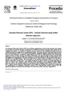
5.3. Precision of Detection 5.3.1. Target Environment To verify the effectiveness of our methodology, we evaluated the detection accuracy by comparing it with other methodologies. We chose two cases for illustration, SQL injection and buffer overrun. Buffer overrun is one of the most popular hacking attacks and a common cause of malfunctioning software. If the amount of data written into a buffer exceeds the size of the buffer, the additional data will be written into adjacent areas. We developed a vulnerable echo server which had a rather small buffer. When we overran the buffer by sending it large amounts of data, the echo server went into an infinite loop. We evaluated our system by detecting this anomaly attack by analyzing resource usage of the echo server process. SQL injection is a technique that exploits the security vulnerability of a PHP script that occurs in the database layer of an application. In our setup, we deployed a vulnerable PHP script and read large volumes of data from the database that should not be accessible, by injecting SQL queries. The vulnerable PHP core was ” SELECT * FROM table WHERE name = ’ ’ ” that can easily pass extended commands such as ’ OR ’1’= ’1’ as a true case for reading all of the database information. We evaluated our system by detecting this anomaly in the resource usage of the Apache (server) process.
Figure 2. Test Environment with Fault Injections
47
International Journal of Security and Its Applications Vol. 3, No. 3, July, 2009
5.3.2. Comparison To demonstrate the effectiveness of our approach, we compared our Hidden Markov Model (HMM) with popular methods such as the Threshold, the Moving Average, and the Rate of Change methods. The threshold method observes CPU usage to determine whether it exceeds a certain threshold. The moving average method sets a sampling period to calculate the average of resource usage dynamically. It also compares the result to a certain threshold value. Rate of Change observes whether the increase in the rate of CPU usage exceeds a threshold. We evaluated each method and selected the best threshold for each by comparing multiple threshold values. A is used for the best threshold value to detect the SQL injection, and B for buffer overrun. The results are shown in Table 6. Table 6. Method and Best Suited Threshold Threshold (A) SQL Injection 0.15 0.09 300.00
Method
Threshold Moving Average Rate of Change
(B) Buffer Overrun 0.35 0.15 5.00
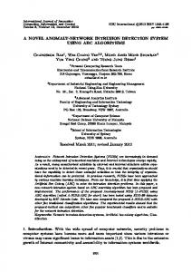
Table 7. Method and Best Suited Threshold Method HMM Threshold A Threshold B Moving Average A Moving Average B Rate of Change A Rate of Change B
SQL Injection Fp Total 0 6 6 4 3 7 20 0 20 3 3 6 20 0 20 0 957 957 0 972 972
Fn
Figure 3. Comparison of Detection Accuracy in SQL Injection
Fn
Buffer Overrun Fp Total 0 2 2 0 5 5 1 0 1 0 5 5 0 0 0 0 27 27 0 27 27
Figure 4. Comparison of Detection Accuracy in Buffer Overrun
5.3.3. Experiments with precision We compared the detection capabilities of each method by using the threshold parameters. We used a system that has learned normal patterns, then we used this experimental environment for evaluation. In the case of SQL injection, we developed a client application that issues SQL queries against the database of the server application. The client accesses the server 1,000 times within 100 minutes. We set up the client to issue attacks 20 times within the above accesses.
48
International Journal of Security and Its Applications Vol. 3, No. 3, July, 2009
This means 2% of the data contains an anomaly pattern. The evaluation criteria are to detect anomalies within three seconds after the server has sent the last message as a response from the client that sent the attack. In the case of buffer overrun, we also developed a client application that uses an exploitation of the vulnerability. The client sends 50 normal messages, then sends an attack message. If Ayaka detects the anomaly within three seconds after the client issues the attack access, it was judged as a success. We evaluate the above case twice. In both cases, we judged a false negative if they could not detect the anomaly within the time limit, and a false positive if they detect the anomaly before or after the limit. We also judge a false positive if they detect a normal access as an anomaly. The results expressed in the number of false negatives (Fn) and false positives (Fp) are shown in Table 7 and Figures 3 and 4. For SQL injection, the HMM, Rate of Change A and Rate of Change B methods show that the number of false negatives are zero (minimum). Even though the minimum number is shown for Rate of Change A and Rate of Change B, the numbers of false positives are 957 and 972. So their total number is same as the false positive. The number of false positives is zero in Threshold B and Moving Average A, B, however, the number of false negatives is 20. This means they have not detected any anomaly in the past. Compared to the total number in the evaluation, both HMM and Moving Average A scores are the minimum, 6. But, when thinking about the detection rate, a false negative of 0 is more important than a false positive of 0, because it means HMM can detect all anomalies. 5.3.4. Precision and Sampling Period In this section, we evaluate the essential factor that influences the accuracy of anomaly detection. We chose the two parameters, precision p and sampling period. We mentioned in section 3 that the precision p has an effect on the accuracy of detection, which is the sum of the probabilities that match the HMM and input data. We consider that the sampling period T also has some effect on the accuracy of detection. We evaluated differences in detection accuracy for these parameters. We took the same procedure as that explained in 5.3. The thresholds are used in both the learning time and detection time, as we described in section 3.3. We set the matrix in which {10-1, 10-2, 10-3} is used to set a different pattern. The results Table 8. Detection Accuracy with Different Thresholds Threshold (Learning) 10-1
10-2
10-3
Threshold(Detection) 10-1 10-3 10-5 10-1 10-3 10-5 10-1 10-3 10-5
Fn 0 0 0 0 0 0 0 0 0
Fp 635 10 6 170 13 13 51 15 15
Table 9. Detection Accuracy with Different Sampling Periods Sampling Period (milisec) 10 100 1,000 10,000
Fn 0 0 0 2
Fp 955 0 6 70
49
International Journal of Security and Its Applications Vol. 3, No. 3, July, 2009
are shown in Table 8. In the results, every combination can detect the anomaly, and lower threshold values show fewer false positives. False positives are lower, especially when the learning threshold is high and the detection threshold is below 10-3. Next, we evaluated the differences of the sampling period and the accuracy of anomaly detection. The results are shown in Table 9. A sampling period of 100ms is the best because false negatives and false positives are zero. For longer periods above 100ms, the number of false negatives and false positives is worse. In contrast, shorter periods (10ms) clearly increase the number of false positives. Considering Table 5, a period of 100ms can achieve the best results with respect to overhead and accuracy of detection.
6. Discussion For our approach, there are two important points to discuss. First of all, our approach uses resource usage (CPU, memory, and network resources) of specific processes to create models with a self-learning approach. In contrast to the existing approaches which use function calls and system calls as information to create the models to detect anomalies, our approach is more general and independent from both language and operating systems. The differences are not so small when we consider developing new embedded system products that are constructed with a variety of hardware and software. For these products, our approach brings benefits to reduce the development time. Actually, there are tradeoffs between accuracy and generality. System calls and function calls have a dependency on their application and operating system, but at the same time, they can provide more specific hints to detect the cause of the anomaly [16]. Moreover, the function calls provide more accurate hints than system calls because of their program dependencies. But, in addition to the accurate results, they provide the larger overheads than the system calls [20]. We think that detecting the cause of the problem accurately with a self-learning method is still not easy, because we could not create all of the anomaly models. We assume that it is better to find an anomaly earlier and in a general way, and it is more practical to analyze the cause manually soon after finding the anomalies. This is the discussion point behind building a practical system. As our next step, we will consider a co-operative system that can offer a log as a complement for our system. The second discussion point is that we need to find the elemental hints for detecting anomalies in our system rather than with the resource data. There are lots of hints to detect anomalies to increase our detection rate. For example, we assume a higher threshold is favorable in the learning phase rather than in the operating phase, because it will generate a new model with less probability than the lower threshold. On the contrary, if we set a higher threshold in the runtime analysis phase, the judgment is more severe when judging it to be normal. We try to find the appropriate threshold evaluation. The results show that our assumption is approximately right on reducing the false positives. It means that our approach still has room to increase the preciseness of detecting anomalies by detecting the relevant parameters. We must try to discover these parameters to increase the detection rate.
7. Conclusion Anomaly detection for future information appliances is a big concern in the area of embedded systems. In this paper, we firstly described the system requirements of current information appliances that are needed for lightweight online monitoring system, and based on their requirements, proposed Ayaka. It is a light-weight anomaly detection system based on resource monitoring of CPU, memory and network usage, independent of programming language and platform. To improve detection accuracy, we use statistical techniques that treat
50
International Journal of Security and Its Applications Vol. 3, No. 3, July, 2009
the data. Our main contribution is to present methodologies to find unknown anomalies without a preexisting strict model of anomalies. We adapt the machine learning technique to study a domain specific model in order to detect anomalies without domain specific knowledge of the system. In our evaluation, the system overhead is about 1.1-1.2%. And for SQL injection, our system presented the minimum number of false negatives and false positives compared to other methods. However, in buffer overrun problem settings, the moving average approach is better than our methodology. This means that the accuracy of detecting anomalies depends on the behavior of the problem. We also find that accuracy was influenced by sampling parameters and thresholds of precision in HMM, within the learning and runtime analysis phases. In the future, we will try to improve our method to detect anomalies more precisely.
Acknowledgement This research was supported by CREST of the Japan Science and Technology Agency (JST), through a Dependable Embedded Operating Systems for Practical Use grant.
References [1] 2009 CBS Interactive Inc. Step-By-Step: How to audit file and folder access to improveWindows 2000 Pro security. http://www.cyberciti.biz/tips/linux-audit-files-to-see-who-made-changes-to-a-file.html. [2] M. K. Aguilera, J. C. Mogul, J. L. Wiener, P. Reynolds, and A. Muthitacharoen. Performance debugging for distributed systems of black boxes. In SOSP ’03: Proceedings of the nineteenth ACM symposium on operating systems principles, pages 74–89, New York, NY, USA, 2003. ACM. [3] D. Anderson, T. Frivold, A. Tamaru, and A. Valdes. Next Generation Intrusion Detection Expert System Operators Manual. Space and Naval Warfare Systems Command, 6 1994. [4] J. P. Anderson. Computer security threat monitoring and surveillance. Technical Report Contract 79F26400, James P. Anderson Co., Box 42, Fort Washington, PA, 19034, USA, 1980. [5] G. Anup and S. Aaron. A study in using neural networks for anomaly and misuse detection. In SSYM’99: Proceedings of the 8th conference on USENIX Security Symposium, pages 12–12, Berkeley, CA, USA, 1999. USENIX Association. [6] P. Barthelmess, J.Wainer, and D. De. Workflow modeling. IEEE Transactions on Software Engineering, 13:222–232, 1995. [7] E. L. Baum and T. Petrie. Statistical inference for probabilistic functions of finite state markov chains. Annals of Mathematical Statistics, pages 1554–1563, 1966. [8] M. Y. Chen, A. Accardi, E. Kiciman, J. Lloyd, D. Patterson, O. Fox, and E. Brewer. Path-based failure and evolution management. In Symposium on Networked Systems Design and Implementation, pages 309–322. USENIX Association, 2004. [9] M. Y. Chen, E. Kiciman, E. Fratkin, A. Fox, O. Fox, and E. Brewer. Pinpoint: Problem determination in large dynamic internet services. In Proceedings of International Conference on Dependable Systems and Networks (DSN), pages 595–604, 2002. [10] M. Desnoyers and M. R. Dagenais. The lttng tracer: a low impact performance and behavior monitor for gnu/linux. In Proceedings of the Linux Symposium, volume 1, pages 209–224, 2006. [11] E. Eskin. Anomaly detection over noisy data using learned probability distributions. In Proceedings of the International Conference on Machine Learning, pages 255–262. Morgan Kaufmann, 2000. [12] E. Eskin, W. Lee, and S. J. Stolfo. Modeling system calls for intrusion detection with dynamic window sizes. In Proceedings of DARPA Information Survivabilty Conference and Exposition II DISCEX, 2001. [13] N. Habra, B. L. Charlier, A. Mounji, and I. Mathieu. Asax: Software architecture and rule-based language for universal audit trail analysis. In Proceedings of ESORICS’92, European Symposium on Research in Computer Security, November 1992. [14] D. Herve, B. Monique, and S. Didier. A neural network component for an intrusion detection system. In SP ’92: Proceedings of the 1992 IEEE Symposium on Security and Privacy, page 240,Washington, DC, USA, 1992. IEEE Computer Society. [15] J. Hochberg, K. Jackson, C. Stallings, J.F.McClary, D. DuBois, and J. Ford. Nadir: An automated system for detecting network intrusions and misuse. Computers & Security, 12(3):235–248, May 1993.
51
International Journal of Security and Its Applications Vol. 3, No. 3, July, 2009
[16] S. Hofmeyr, S. Forrest, and A. Somayaji. Intrusion detection using sequences of system calls. J. Comput. Secur., 6(3):151–180, 1998. [17] K. Ilgun. Ustat: A real-time intrusion detection system for unix. In SP ’93: Proceedings of the 1993 IEEE Symposium on Security and Privacy, page 16, Washington, DC, USA, 1993. IEEE Computer Society. [18] K. Ilgun, R. A. Kemmerer, and P. A. Porras. State transition analysis: A rule-based intrusion detection approach. IEEE Transactions on Software Engineering, 21:181–199, 1995. [19] Information-technology Promotion Agency, Japan. Current Security Issues and Strategies in Embedded System. http://www.ipa.go.jp/event/ipaforum2007/program/pdf/isec-Ukai.pdf. [20] M. Keith. Analysis of computer intrusions using sequences of function calls. IEEE Trans. Dependable Secur. Comput., 4(2):137–150, 2007. [21] S. Kumar and E. H. Spafford. A pattern matching model for misuse intrusion detection. In Proceedings of the 17th National Computer Security Conference, pages 11–21, 1994. [22] J. B. MacQueen. Some methods for classification and analysis of multivariate observations. In Proceedings of the Fifth Berkeley Symposium on Mathematical Statistics and Probability, volume 1, pages 281–297. University of California Press, 1967. [23] nixCraft. Linux audit files to see who made changes to a file. http://www.cyberciti.biz/tips/linuxaudit-files-tosee-who-made-changes-to-a-file.html. [24] A. Pedro, Diaz-Gomez, and D. F. Hougen. Improved off-line intrusion detection using a genetic algorithm. In ICEIS (2), pages 66–73, 2005. [25] A. Phillip, P. Porras, and G. Neumann. Emerald: Event monitoring enabling responses to anomalous live disturbances. Technical report, SRI International, Menlo Park, CA 94025, 1997. [26] K. Sandeep and S. Eugene. An application of pattern matching in intrusion detection. Technical Report 94013, Department of Computer Sciences, 1994. [27] A. Stefan. Intrusion detection systems: A survey and taxonomy. Technical Report 99-15, Chalmers Univ., March 2000. [28] M. Sugaya, S. Oikawa, and T. Nakajima. Accounting system: A fine-grained cpu resource protection mechanism for embedded system. In Proceedings of the 12th Internaltional Symposium on Object/component/service-oriented Real-time distributed Computing (ISORC), pages 72–84, 2006. [29] Sun Microsystems, Inc. Trusted Solaris Audit Administration, November 2001. [30] C. Warrender, S. Forrest, and B. Pearlmutter. Detecting intrusions using system calls: Alternative data models. IEEE Symposium on Security and Privacy, 0:0133, 1999.
52
International Journal of Security and Its Applications Vol. 3, No. 3, July, 2009
Authors
Midori Sugaya is a researcher of Dependable Embedded OS R&D Center, Japan Science and Technology Agency (JST). She has eight years of work experience in the software industry. She received Master Degree in computer science from Waseda University, Japan, 2004, and also a candidate of the PhD in computer science from Waseda University. Her research interests include operating and dependable systems and proactive fault management system.
Yuki Ohno received a B.S. degree in computer science from Waseda University, Japan, 2008, and now he is a master's student in the Department of Computer Science at Waseda University, Japan. His research interests are in monitoring, operating system and resource management in distributed system. Tatsuo Nakajima is a professor of Department of Computer Science and Engineering in Waseda University. His research interests are embedded systems, distributed systems, and ubiquitous computing. His research group is developing advanced software infrastructure for future many core processors for embedded systems and future ubiquitous computing services.
53
International Journal of Security and Its Applications Vol. 3, No. 3, July, 2009
54