some other piece of software. Loosely analogous to a âhardware componentâ such as a screw or a gear-box, a software component has clearly defined char-.
Lightweight Component Models for Embedded Systems∗ H. John Reekie and Edward A. Lee Dept. of Electrical Engineering and Computer Science University of California at Berkeley
Abstract Components are receiving attention as a means of advancing the state of software distribution beyond the traditional choices of source code, compiled binary executable, and compiled libraries. In this paper, we examine lightweight component models for embedded real-time software systems, and propose two different component models based on the concepts of actors and models of computation.
1
Introduction
We are exploring the concept of software component [17] in the context of embedded and real-time systems. Although the term “component” is used in many different ways, the term is coming to have an established meaning in software design and implementation, and we follow the emerging usage of this term. Intuitively, a software component is a piece of software that can be “plugged into” some other piece of software. Loosely analogous to a “hardware component” such as a screw or a gear-box, a software component has clearly defined characteristics and clearly defined behavior in the domain of interest. In addition, the context of production and consumption may be quite different (analogously, the manufacturer of a screw does not know to what use the screw may be put). In the embedded systems realm, performance and predictability often outweigh reusability as key concerns in system construction. As a result, even systems that are modeled and designed using sophisticated techniques and modeling tools are built largely “by hand.” We see the adoption of software component models specifically designed for embedded systems as one way of improving the ability to “bridge the gap” from systems modeling efforts to implementation. In the Ptolemy Project, we have been exploring systems modeling using actors and models of computation for some time [4]. We suggest in this paper that these principles can be adapted to component models targeting real-time embedded systems. We will first give a brief overview of software components ∗ Published as Technical Memorandum UCB ERL M02/30, Electronics Research Laboratory, University of California at Berkeley, October 2002.
1
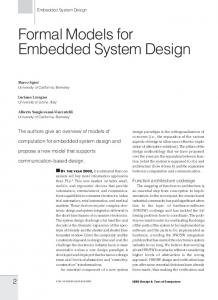
as we see them, and explain why actor-oriented software design is a natural choice for embedded systems components. We will then describe two lightweight component models that explore different parts of this space. Software components Szyperski defines software components to be “binary units of independent production, acquisition, and deployment that interact to form a functioning system” [17]. He clarifies that “binary” means any format that can be executed by the target machine [18]. This may be code for a specific processor, or virtual machine code, or in some cases even source code (as in some scripting languages). Figure 1 illustrates a possible component scenario. The source code of a component is compiled to generate the two parts: the component interface, and the component “binary,” or executable portion. At a later time, multiple components are assembled together and loaded onto a target platform for execution. The target platform typically contains some kind of runtime support, which we have shown in the figure as the component runtime. In some component models, a separate entity called a controller may exist to coordinate the activities of the components; the controller may be a pre-written module, or may even be synthesized by the component assembler. The collection of all of these pieces of software is called a component framework. In a component world, therefore, we add to the traditional notions of designtime, compile-time, and run-time, the notion of assembly-time. In some cases, “assembly” of a component is done at run-time—such is the case with browser plug-ins, for example. In others, it is done on a machine different to the target machine, as the final step in the development of the program. We use the term component model to mean a description of components and a component framework that abstracts from the details of a concrete implementation, such as the exact format of the component executable. Our goal in doing so is to understand the choices that can be made in the design of a component architecture, without getting distracted by machine- or platform-specific details. This is doubly important in embedded systems, as we believe that the diversity of process and system architectures will mean that many different implementations of any given component model will be needed. A component model defines, among other things, the structural elements of its components. Typically, a component will have a set of method calls, often grouped into implementations of sharable method interfaces. Some component models support events, whereby a component offers to notify other components when some particular event occurs. The event mechanism may be explicitly declared (as in the Corba Component Model [16]), or implicit in stylized method and type signatures (as in JavaBeans [6]). Components may also depend on the presence of other components. This can lead to tight sets of dependencies between components—a component may require the presence of a particular database server component, for example. Szyperski remarks that such dependencies are not uncommon in coarse-grained component models [18]. 2
Controller
synthesize compile
actor { }
Source code
Component runtime Interface
Executable
assemble Executable components
Component
Target platform
Figure 1: Component usage Component executables Figure 2 illustrates a possible set of transformations that might be performed on the executable part of a component. A component starts off in a hand-written source form, and ends up in a machine-executable form. Along the way, it may progress through a core language, an intermediate form (IF), and a virtual machine code. Any point along this chain could potentially be chosen as the component’s “executable” format; the component assembler and run-time will then provide the rest of the path to execution. For example, if we chose an IF as the executable format, then one path to execution would be a code generator to a virtual machine, and a VM interpreter. If we chose virtual machine code, then we can either interpret that directly, or compile it to native code and run it on an appropriate instruction unit. This diagram illustrates the tradeoff in choosing the form of components. By choosing a point further towards the left, we place a higher burden on the component assembler or run-time. For example, if we choose to deploy components as source code, then the author of the component assembler is obliged to include a component compiler and optimizer. We also run greater risk of accidentally introducing unwanted dependencies on external source code. If we choose a point further to the right, the burden on the component assembler is reduced, at the potential cost of lost optimization opportunities. Component interfaces In general, a component should carry or have bundled with it information that enables a potential client to decide whether and how to use it. This information we clump under the heading of “interface”—the interface tells the client or component assembler everything there is to know about the component, other than the exact procedure by which it performs its work—that is “hidden” in the executable. Potentially, a complete component model might include version in3
Compile
Transform
Source
Codegen
Compile
Core
Codegen
Intermediate form
push push add
Native CG
VM code
load r0 load r1 add r0,r1
Native code
VM Interpreter Interpreter
Instruction unit
Executing code
Figure 2: Transformation of a component executable formation, author and vendor information, identity authentication, performance and cost metrics, usage documentation, and test vectors. Current component models do not have strong interfaces, being mostly limited to static type signatures. A stronger form of component interface is an assume-guarantee interface. Type signatures and assume-guarantee interfaces are an example of stateless interfaces, since the interface specification does not depend on the runtime state of the component. In the context of embedded systems, other types of stateless interface will need to be supported, such as timing information, resource usage, and so on. A more powerful and comprehensive approach to component interfaces is given by Alfaro and Henzinger’s interface theories [3]. In general, an interface of a component might be stateful, that is, it captures dynamic behavior of a component. For example, a stateful interface for a file server component will insist that a file be opened before it is read. Interface automata [2] are an example of stateful interfaces. Stateful interfaces are a general means of capturing the “semantic information” that have been proposed briefly for components for general-purpose computing [13]. A component framework must ensure that component interfaces are respected. Ideally, this would be performed once, at assembly-time—type systems are the classic example of this. Since a static check is not always possible, the component assembler may generate code to monitor the component at run-time and raise a run-time exception if an interface is violated. Assertions in C are a crude example of this type of checking.
4
2
Actor-oriented components
Actor-oriented software design [9] is an approach to systems design in which entities called actors communicate through ports and communications channels. Actor-oriented design is a natural match to embedded systems. One reason for this is that embedded systems designers are well-versed in notations and concepts that lend themselves to “box-and-arrow” notations, such as signal processing block diagrams, state machines, and so on. Another is that this style of program construction does not over-specify the program by requiring the programmer to explicitly sequence the operations of the program. Finally, efficient schedules for actor execution can often be automatically derived.
2.1
Actors and models of computation
In an actor-oriented software framework, the interaction between actors is captured by what is known as a model of computation. Abstractly, a model of computation is a description of the interaction and communication between actors. Formally, it is a description of relations between tagged signals [12]. At the implementation level, it is an algorithm for sequencing the flow of control through a set of actors, and data structures that represent the appropriate form of actors and communication channels. Examples of different models of computation include discrete-time, dataflow, and continuous-time models. These and a large number of other models of computation suitable for embedded systems design have been explored in the context of the Ptolemy project [8]. The key thing to note about models of computation in an implementation context is that control flow is removed from the actors. This has important implications for a component model based on actors. Let’s consider an example. Suppose we have two processes, with the output of the first connected to the input of the second by a FIFO queue. We could write them as in Figure 3. By doing so, we have specified a key operational detail of this program that, really, we didn’t need to: this program requires a multi-threaded environment with context-switching in which to run. Suppose we now re-factor the program as in Figure 4. This version of the two processes still requires a multi-threaded environment, but by separating the control flow— that is, the threads—from the computation contained in the actors, we have enabled other models of computation to be employed with the same actors. For example, we can now write a “dynamic dataflow” (DDF) program as in Figure 5, where actors A and B are as before, and process C is a single-threaded DDF controller for that network. Finally, in this particular example, we know that actor A produces one token each time it fires, and that actor B consumes two tokens each time it fires. This is the synchronous dataflow (SDF) model of computation [10], and a schedule can be computed for a network of such actors. In this case, it would result in the controller shown in Figure 6. As seen by this example, we are “lifting” control flow out of the actors and into an external entity (the controller). In comparison, other component models tend to place the control flow inside components. Apart from the thread 5
process P { forever do { wait for a token on the input channel read the token into variable x write f(x) to the output channel } } process Q { forever do { wait for two tokens on the input channel read the tokens into variables y and z write g(y,z) to the output channel } } Figure 3: Two processes
process P { forever do { wait for a token on A’s input channel fire actor A } } process Q { forever do { wait for two tokens on B’s input channel fire actor B } } actor A { read a token into variable x write f(x) to the output channel } actor B { read two tokens into variables y and z write g(y,z) to the output channel } Figure 4: The same two processes, refactored
6
process C { forever do { if there is a token on A’s input channel fire actor A if there are two tokens on B’s input channel fire actor B } } Figure 5: A DDF controller for the two-process network process C { forever do { fire actor A fire actor A fire actor B } } Figure 6: An SDF controller for the two-process network example above, consider a model with an event subscription and notification model, such as JavaBeans. When an event is generated, the notification of the event is implicitly a transfer of control—in this model, control tends to follow the data. By removing control flow from actors, we are able to make the same actors usable in multiple execution contexts—we have not constrained their use by unnecessarily specifying the use of threads, for example. We have also opened opportunities for performance optimizations—by removing context switching and by applying static analysis to determine schedules, for example. We have also created verification opportunities, since we now have more control over the behavior of the network of actors and are thus better able to make statements about the performance and predictability of the network. Finally, we have simplified the implementation of the components themselves, as will be shown in the following sections.
2.2
Actors as embedded systems components
In general, we think that component models will become more domain-specific than the current general-purpose models. By restricting the scope of a component model, components become easier to compose and verify. In the embedded systems realm, we believe that actors are a good choice for “componentizing” embedded systems software: the use of functional blocks connected by edges that represent some kind of flow of data is a good match to many forms of
7
embedded systems specification, as mentioned already. Other parts of a component framework could also be “componentized” (schedulers, for example), but we have not addressed this in this paper. An actor typically consists of three main elements. First, a set of methods that are shared by all components and are used by the component framework to perform operations common to all actors. Typically, these operations will perform functions like initializing and shutting down the component, and for this reason we refer to them as life-cycle methods. Second, one or more actions, each of which processes input data to produce output data. Third, a set of parameters which are used to control operation of the actor by an external entity such as a user interface. In the following paragraphs we will look at some generic issues in component models for embedded systems. Encapsulating hardware Components are a natural match for encapsulating hardware interfaces. Embedded systems programmers must often deal with low-level code such as interrupt service routines (ISRs) and data buffering. Consider a driver for an analog I/O device interfaced to a DSP (digital signal processor). The interface might be implemented using an off-the-shelf A/D/A converter chip, with which the DSP communicates using an on-board serial port. The driver for this interface needs to communicate with: a) the lowlevel hardware and b) the higher-level processing software. (a) might involve setting memory-mapped registers that configure the serial port, sending a series of control words to the A/D/A chip, and installing one or two interrupt service routines (ISRs) to handle the serial port interrupts. (b) requires that the driver implement an intermediary layer between the ISR and the higher-level code. In a real-time DSp application, the ISR must be as short as possible (tens of microseconds); as a result the driver must be structured so that most of the work be done when the client calls, not in the ISR itself. In a component world, the “driver” for the analog interface is encapsulated into a component, as illustrated in Figure 7. The component model must have the mechanisms to support the notion of components that synchronize to real time.1 Provided this is done well, the component assembler is able to combine components from different sources (for example, those provided by the hardware platform vendor, those purchased from a third-party software supplier, and those written in-house), without regard to platform-specific idiosyncrasies. Execution, likewise, uses the same infrastructure for all components, without having to have code hand-written by a programmer to different device-specific APIs. 1 We have not addressed this issue in either of the component models presented in the rest of this paper. This is a subject for further discussion and a future paper.
8
Actor interface
init {
fire_a {
}
}
Control registers Buffers Read ISR Jump table Write ISR
Figure 7: A component that encapsulates hardware Binary components Referring back to Figure 2, on the question of which format to choose as the distribution format of a component, we lean towards the right-hand side of that figure—that is, to the lower-level formats like native machine code. One could argue that distributing components in source code format leaves better opportunities for optimization (by merging components and converting channel reads and writes into simple variable access). Nonetheless, binary-format distribution does have advantages: • It enables protection of proprietary information, which is essential if vendors of algorithms for specific hardware platforms are to provide software in component form. (Currently, signal processing algorithms are typically provided as binary function libraries.) • It enables multiple source languages to be used. A number of DSP vendors have produced excellent C compilers tuned to the architecture of their DSP devices, and have added extensions to enable even better performance to be obtained from the device. Expecting to be able to reproduce these device-specific optimizations in some “common” source language is unrealistic. • Finally, we believe a binary component format encourages independent component development. By focusing on producing binary components with a small and very well-defined interface, independently of any particular execution context, those components will be better suited for use in multiple contexts. 9
word num
addr array
struct
int
float
Figure 8: An example type lattice, for a typical 32-bit floating-point processor Taken individually, none of these may be particularly compelling, but taken together, we think they point to binary formats as the preferred primary means of distribution of components for embedded systems. Polymorphism and parameterized types If a low-level executable format is chosen, it is likely that the executable code in the components will not be polymorphic. For example, in a high-level language, we might write an add method that has a type signature add : (num × num) → num (where num is a supertype of various numeric types). While convenient for the programmer, this is not feasible in a component distributed in machine code for a particular processor, particularly if we are concerned with efficient embedded implementation. We therefore suggest that a component suitable for embedded systems provide for multiple implementations of each entry point, specialized to concrete low-level types. A convenient way to handle this is to give the component model a parametric type system, such as in Haskell [7], which structures types into a lattice such as shown in Figure 8. Method types are declared using type variables, for example: add : num α ⇒ (α × α) → α Here, the type variable α represents any concrete type that can represent num, that is, any leaf below num in the type lattice. Each specialized implementation would then be tagged with the instantiated type variable—α = int or α = float, for instance. The component assembler will choose a particular concrete implementation according to the context in which the component is used.
3
The Actif component model
Actif is the first of two component models proposed in this paper. It has a separate executable and interface, and a controller that is synthesized from the component interfaces. We believe that Actif will prove to be a powerful tool for building reliable real-time systems. In this section, we present the basic
10
elements of this model. There are aspects of the model that we have not yet finalized, such as the representation of time and synchronization with real time; these are topics for a future paper.
3.1
Actif components
Lee and Parks introduced the notion of firing rules to govern execution of a dataflow process [11]. In their formulation, an actor has one or more firing rules, each of which contains a set of patterns (one per input channel) that are matched against the data present on the input channels. If all patterns match, then that action can be fired. For example, an actor that reads a single token from each of two inputs has the firing rule R1 = {[∗], [∗]}. The pattern [∗] will match an input channel if the channel contains at least one data value. Lee and Parks allow constants to appear in firing rules. For example, an actor that selects from one input or another according to the boolean value on a third input has two rules: R1 = {[∗], [], [F ]} R2 = {[], [∗], [T ]} That is, if the token on the third input is false (F ) and a token is present on the first input, the actor reads it. If the token on the third input is true (T ) and a token is present on the second input, the actor reads from that input instead. (The pattern [] always matches.) In Actif, we adopt a similar notion: an actor consists of a set of actions, each of which has a firing rule. We do not, however, allow constant values in firing rules—as a result, an action can be fired based only on the number of tokens present on the input channels. Sequencing between actions is constrained by a firing automaton; this is in contrast to Lee and Parks, who provide an algorithm to determine whether a set of firing rules is sequential, and if so, to determine a unique order in which the rules can be tested. Actif is a refinement of a dataflow model called “phased dataflow” that was proposed in [15]. In more recent work, the Cal actor language [1] also uses multiple guarded actions, but these are considerably more sophisticated than Actif’s firing rules. For the purposes of exposition, we hereby invent a small “C-like” language for describing actors. We are not proposing this as a necessary part of Actif, it is just a convenient means of describing actors in sufficient detail that we can talk about the component model. In this language, we would write the add actor like this: actor add (float in1, float in2) (float out) { action a ([x][y] -> [x + y]); } This actor has two input channels, in1 and in2, and one output channel, called out. All channels carry numbers of type float. The single action a reads a value from each input channel and writes the sum to the output channel. The firing 11
* b
*
p
a (a) add
c
a ¬p
(b) select
a
*
b
(c) merge
Figure 9: Firing automata: a) add, b) select, c) merge automaton of this actor is shown in Figure 9a; in this case, as with any actor with a single action, the automaton has a single state and a single transition, and is trivially derived from the actor. In general, a firing automaton has two types of vertices, called place vertices and choice vertices, and two types of transition, called action transitions and choice transitions. A place vertex represents the state of an actor between executing actions. Action transitions leave place vertices and represent execution of an action. Choice vertices, colored black, represent a branch in control flow, where the actor decides which place vertex to proceed to after completing an action. Choice transitions leave a choice vertex and are labeled with a boolean expression. Consider the select actor. Its firing automaton includes a choice vertex, which determines which action the actor is prepared to execute after reading the control token. The actor would be written like this: actor select (word in1, word in2, boolean ctrl) (word out) { action a ([][][p] -> []) next (if p then b else c); action b ([x][][] -> [x]) next a; action c ([][y][] -> [y]) next a; } The firing automaton of this actor is shown in Figure 9b. In comparison to the Lee/Parks firing rules, this actor needs an extra action (the one labeled a) to perform the read of the boolean value; this extra action is, in effect, making sequentialization of the firing rules explicit. 12
actor mac (float in) (float out) { parameters { float factor = 1; } state { float current = 0; } action a ([x] -> [y]) { y = current + factor * x; current = y; } } Figure 10: The mac actor If a place vertex has more than one output transition, then the transition taken is chosen non-deterministically. For example, the merge actor, with firing automaton shown in Figure 9c, can non-deterministically choose to read from either input: actor merge (word in1, word in2) (word out) start a,b { action a ([x][] -> [x]) next a,b; action b ([][y] -> [y]) next a,b; } In this example, the start clause states which set of actions should be initially considered. The start and next clauses contain sets of actions, meaning that any action in the set will be considered for execution. None of the actors so far have parameters or state. Figure 10 shows the mac actor, which has a parameter factor and a state variable, current. It multiplies each input value by a constant factor, and adds the product to the previous output value. It is smaller than we would normally expect components to be, but serves well enough as a concise example for the following sections.
3.2
Component structure
Actif actors are compiled into separate executable and interface portions. In the executable portion, each action is implemented by a single procedure. The argument to this procedure is a pointer to a block of memory that contains the instantiated component’s parameters, state, and input variables. The procedure computes output values and new state values from the inputs, and writes them to the memory block. To illustrate, we will assume that the component compiler generates C code, which can then be compiled again to produce the executable portion of the 13
struct mac_vars { float current; float factor; float x; float y; } void fire_mac_a (struct mac_vars *vars) { vars->y = vars->current + vars->factor * vars->x; vars->current = vars->y; } Figure 11: The executable portion of mac, when compiled to C component. Figure 11 shows the C code generated by the component compiler for the mac actor. As you can see, it’s a fairly straightforward translation of the component source code. Figure 12 illustrates the code generated by the component assembler to call an instance of the mac actor. Again, we assume that the output of the component assembler is C code, which is then compiled to produce an executable controller. The interesting part of this code is the three lines at the end: it reads an input value and writes it to the memory block vars; it then calls the action procedure fire mac a; when that returns, it reads the computed output value from vars and writes it to the output channel. The interface part of the component must contain sufficient information that the assembler can generate this code. Figure 13 illustrates a possible interface for mac in an XML language. It contains all of the information in the actor definition, except for the actual computation that is performed by the action— that part of the actor is kept hidden from the component assembler. To summarize, each actor has a single structure containing parameters, state variables, input values read from the input channels, and computed output values. Each action of that actor has a single procedure that accepts a pointer to that structure as its argument. We highlight a few points about the model: • The actor is not responsible for reading input from channels or writing output to channels. This is handled by the code synthesized by the component framework. This approach removes the need for polymorphic interfaces to a channel, as in systems such as Ptolemy II. • In some coordination models, actors are expected to not update their state when they produce output. In Actif, this means that the controller must make a copy of state that is modified by an action and restore it after the action completes. In addition to the code generated for the actions, all components have several life-cycle methods:
14
struct mac_vars { float current; float factor; float x; float y; } struct mac_vars mac_0_vars = { 0.0, 1.0 }; extern void fire_mac_a (struct mac_vars *); extern struct inputChannelFloat *mac_0_input; extern struct outputChannelFloat *mac_0_output; ... mac_0_vars_a.x = readInputFloat(mac_0_input); fire_mac_a(&mac_0_vars); writeOutputFloat(mac_0_output, mac_0_vars_a.y); ... Figure 12: Sample code generated to call mac, in C
Figure 13: The mac interface
15
• initialize is called when the component is initialized. It can allocate memory needed by the actor, initialize registers on peripheral devices, install ISRs, and so on. • reset returns the actor to the state it was in just after initialize was called. • finalize shuts down the component. It can release memory, disable peripheral devices, turn out the lights, and so on.
3.3
Controller synthesis
Once a set of components has been connected into a network, the component assembler needs to synthesize a controller for them. A suitable intermediate form for this controller is a state machine, where transitions represent selection and execution of an action. Let M (α) be a predicate that tests whether an actor has the required tokens on its inputs for action α, and F (α) be the instruction to fire action α. The transition labeled α ∈ A(f ) : M (α)/F (α) means “select an action α from the set of enabled actions of actor f with matching input tokens, and fire it.” For example, Figure 14a shows a simple two-actor network as we used in the example in section 2. Figure 14b is a DDF controller for it: each transition selects an action from actor f or g and fires it. In this case, since there are two transitions from the initial (and only) state, either transition can be non-deterministically chosen. Controllers can also specify a single action to be taken on a transition. We write this as, for example, M (fa )/F (fa ), meaning “fire action a of actor f , provided that it has matching input tokens.” Or without the guard, F (fa ) means “fire action a of actor f .” Figure 14c illustrates an SDF controller for the example network, again assuming that f produces one token each time it fires, and that g consumes two tokens each time it fires. (Since the scheduler for the SDF coordination model guarantees that sufficient tokens are available, there is no need to test for the controller to test for the presence of tokens.) In some coordination models, the controller may iterate to a fix-point before updating the state of the components. This requires that the controller preserve the state of the actor prior to firing an action, and restore it if iteration is required. We will refer to these instructions as prsv(fa ) and rstr(fa ). (They are action-specific, as not all actions will modify the whole state, and it makes no sense to preserve parts of the state that will not be modified.) To illustrate, Figure 15a shows a simple continuous-time network that represents the following set of differential equations: x˙ y x(t0 )
= f (x, u, t) = g(x, u, t) = x0
This system has a continuous portion, being the input signal and the loop around f and the integrator, and a discrete part, being the actor g and the output signal. For simplicity, we will assume that f and g each have only
16
1
f
1
2
g
1
(a) A simple model
* b Î A(g) : M(b)/F(b)
F(ga)
F(fa)
* a Î A(f) : M(a)/F(a)
F(fa) (c) SDF controller
(b) DDF controller
Figure 14: A simple network and two controllers for it a single action. To execute this system, the controller, shown in Figure 15b, repeatedly fires f until it is satisfied that the computed continuous value out of the integrator is a sufficiently good approximation. Each time, it must restore the state of f prior to firing it again. When computation of the output value of f converges, the controller moves onto the next phase and fires g.
4
The Compact component model
Compact is the second of our two component models. It is being developed as a lightweight framework for execution of components in Java. Its primary aim is to provide a means by which components developed by different authors can be executed in more than one execution framework, again developed by different authors.
4.1
Overview
One of the issues in building a conventional software framework is coupling between the various parts of the framework. As a design evolves and gets larger, this coupling inevitably becomes tighter and less structured. In an actororiented framework such as Ptolemy II, for example, actors come to depend on numerous APIs for retrieving and sending data, communicating with the execution code for special purposes such as scheduling delayed execution, and various other services. Conversely, the framework comes to depend on various
17
done/F(ga)
u
f
g
ò
y
Ødone/rstr(fa)
* prsv(fa)
step
x
M(fa)/F(fa) (a) Continuous-time model
(b) Controller
Figure 15: A continuous time network and its controller actor APIs, such as a potentially unbounded number of “marker” interfaces or superclasses to indicate that an actor implements some particular type of functionality. A component approach, in contrast, enforces explicit declaration of dependencies. In particular, components can be developed independently of a particular execution framework, thereby reducing the possibility of accidental dependencies between components and a particular framework. Compact is a component model targeted specifically at Java platforms. We have designed this model to be easy to implement and to allow direct authoring of components. Thus, Compact does not have a separate interface portion, nor does it require a component compiler. We therefore don’t consider Compact to be a “proper” component model; nonetheless, we think it will be useful and give us a means of exploring the implications of component models on a broader and more accessible range of platforms. Figure 16 illustrates how Compact mediates between different component sources and execution frameworks. In the first instance, components can be written by hand. Secondly, components could be generated from a Ptolemy II model using the Copernicus code generation tool [14]. Copernicus, by using a technique called co-compilation and some knowledge of the Ptolemy II framework, is in effect able to compile away some of the framework dependencies for us. One interesting consequence of this would be the ability to develop significant IP in Ptolemy II, and then compile it into a more efficient component for execution in other, non-Ptolemy, execution frameworks. Finally, components could be written in an actor definition language such as Cal [1], and compiled to Compact. On the execution side, components can be executed in any execution framework that is able to adapt itself to the Compact component model. We note again a key difference between component models and frameworks: with a suitable component model, components can be developed independently of the final execution environment. We are also designing for Compact its own execution framework, called Clef (for Compact Lightweight Execution Framework). As its
18
Hand-coded actor Ptolemy model
Ptolemy/Ptact Compact component
Cal actor
Clef ?
Figure 16: Compact and its place in the universe name implies, Clef is small and efficient, and as such, is suitable for execution on small platforms or for embedding into other applications. CLEF is capable of being run on J2ME [5], the embedded version of the Java Platform.2 We also plan to experiment with using Clef as an execution engine in a visualization framework, to sequence control flow through complex visualization processing networks. Incidentally, the name “Compact” originated as a contraction of the words “component” and “actor,” but we also like it because it summarizes the philosophy of this model well.
4.2
Component structure
Compact is a Java-specific component framework, and uses the reflection capabilities of Java to encode the interface of a component in the Java source code. We will use the mac actor as our example again—mac in Compact is shown in Figure 17. For each port, the component declares (but does not create) an object of a suitable type. Compact provides a set of interfaces for this purpose. The mac actor, for example, has two double-carrying ports, of type IDoublePort, shown in Figure 18. These ports are instantiated not by the actor, but by the component run-time, thus allowing the run-time to supply different implementations of the port according to the coordination model in which the actor is used. Each component class requires a public static variable called signature, which tells the component assembler which ports are inputs and which are outputs. In addition, it gives for each port the minimum number of tokens consumed by inputs and produced on outputs. If additional tokens are needed then this is indicated by a trailing +; for example, the signature that indicates that an actor reads one or more tokens on the port in, and always produces just one on the port out, is in(1+) -> out(1) 2 Specifically,
we are targeting the version known as CDC/FP, that is, the Connected Device Configuration with the Foundation Profile. This platform is suited for systems with 2MB or more of memory, and does not include graphics capability. Targeting the much smaller CLDC (Connection-Limited Device Configuration) would require a component model more akin to Actif, in which component source is compiled into a form more amenable to execution on a small platform.
19
public class Mac implements IActor { public String signature = "in(1) -> out(1)"; public IDoublePort in; public IDoublePort out; public double current = 0.0; private double _factor = 1.0; public double getFactor () { return _factor; } public void setFactor (double f) { _factor = f; } public void fire () { double x = in.get(); current = current + x * _factor; out.put(current); } } Figure 17: The Mac class written in Compact (There is no special significance to the names in and out; they are just names.) In the mac example, just a single token is consumed and produced. If the token count is omitted, it is assumed to be one. A simple extension to this language, required for multi-rate signal processing actors, would be to allow the token count to be set to the name of a parameter. Actor firing is implemented by the method fire, from the IActor interface. This method reads inputs, writes outputs, and updates the state. The controller guarantees that, when fire is called, the minimum number of input tokens specified in signature are present in the input ports—the actor does not need to check for the presence of this minimum number of tokens, and is in turn obliged to consume at least that many tokens. As in Actif, a firing may modify the actor’s state, so if a controller requires that an actor’s state be preserved in a firing, it must do so explicitly. The actor’s state is assumed by default to be the set of public instance variables; actors can optionally implement an interface called IMemento to gain control over the copying and restoring of their own state. For each configuration parameter, a component has a JavaBeans-like property, indicated by appropriate get and set methods. In the example, factor is such a property. Since reading and writing configuration parameters is an infrequent operation, the component run-time can use reflection to do this. As in Actif, Compact actors can have three life-cycle methods, initialize, reset, and shutdown. These methods are declared by the ILifeCycle interface. If a component does not implement ILifeCycle, then the component run-time will assume that initialize and shutdown do nothing, and will reset the state to its initial value for reset.
20
public interface IDoublePort { int getCount(); double get(); void put (double d); } Figure 18: The port interface for doubles
4.3
Polymorphism
Despite being written in Java, Compact is kept fast and lightweight by using primitive Java data types, without “boxing” them in polymorphic Token objects. Instead, we lay the burden of presenting polymorphism to the user on the component assembler user interface, if desired. Our reasons: • Polymorphism in significant numerical algorithms is often not straightforward. For example, a signal processing filter will need to be written differently for fixed-point and floating-point implementations—the fixed-point implementation requires additional code for overflow checks and scaling operations that are not needed in the floating-point implementation. • Run-time polymorphism can be very expensive. In Ptolemy II, for example, every arithmetic operation makes method calls into the type system to check for type compatibility, and requires allocation of a new object for the result. • If a Ptolemy II model is compiled into a component with Copernicus, then the resulting component will be monomorphic anyway, since the compiler requires concrete types to perform token unboxing, one of its most significant optimizations. In a similar vein, if an actor definition language is used to write components, then a single polymorphic source actor can be compiled into a “family” of Compact components.
4.4
Executing Compact components
Compact components can be executed in any environment that can adapt to its component format. Because this format is so simple, we hope that there will be multiple platforms that will support Compact components, thus facilitating sharing of components between researchers and developers. We will illustrate here how a Compact component could be executed in the Ptolemy II execution environment. Our ideas here are based on recent work on compiling Cal actors to execute in Ptolemy II [19]. Execution of a Compact component in Ptolemy II uses a set of adapter objects, which we have named Ptact. A Ptolemy actor is significantly more complex than a Compact component, and has a high degree of dependency on the various bits and pieces of the Ptolemy API (in contrast to the Compact component, which has none). Specifically: 21
Ptolemy director
TypedIOPort
TypedIOPort Ptact adapter
DoublePort
Compact component
Parameter
DoublePort
Figure 19: A compact component adapted to Ptolemy II • Ptolemy actors communicate using polymorphic Token objects that encapsulate primitive data items, whereas Compact actors read and write primitive data items. • Ptolemy supports multi-threading, whereas Compact does not. • Ptolemy actors support multi-ports—that is, ports that contain multiple channels, but Compact only has ports with single channels. • Ptolemy actors support arbitrary sets of named parameters, whereas Compact components have only a fixed set. Figure 19 shows the structure of a Ptolemy actor, implemented using a Compact component and the Ptact adapters. In this diagram, single arrowheads indicate a reference, and double arrowheads indicate a reference and a calling interface. Grey objects are those that are part of Ptact. The Ptact actor adapter creates the other adapter objects, as well as providing the execution interface to a director (the Ptolemy II equivalent of a controller). Parameter objects read from and write directly to properties of the Compact component. The port adapters mediate between the Compact component and the Ptolemy ports, and perform token boxing and unboxing.
5
Concluding remarks
We believe that, as component models mature, domain-specific component models will arise in various fields. In this paper, we presented our view of components for embedded software systems, and described two different component models based on the concept of actor-oriented software design. The two models deliberately present different choices in the design space of component models for embedded systems. In future, we expect that other component models 22
will be developed that focus on different capabilities. Examples could include component models tailored to system-on-chip hardware design, or to embedded systems that consist of large number of mobile nodes. Of the two component models, Actif is the more substantial, but also the more complex to implement. It requires that components be programmed in a language specific to the purpose, and then compiled to generate executable and interface portions. The controller for an assembled network of components must be synthesized from a description of the network and the component interfaces. Because actions of an Actif component will always consume and produce a known number of tokens, we believe that Actif holds more promise for building dependable and reliable real-time systems. Finally, because Actif has a separate interface, it also provides a ready platform for further research into more advanced interface specifications for embedded systems components. Compact, in contrast, is designed to be simple to implement, and is restricted to one language. It does not require a component compiler, nor does it require that a controller by synthesized for each network. It is therefore intended more as an experimental platform for component models, and as a “half-way” point between a true component model such as Actif, and higher-level modeling environments such as Ptolemy II. We are proceeding with implementations of both component models. The implementation of Actif is the longer-term project. The Compact implementation is shorter-term, and will include the dedicated execution framework Clef, and the Ptact adaptor to allow Compact actors to be executed within Ptolemy II. We hope that we will be able to collaborate with other researchers in embedded systems to provide similar adaptors for their own execution frameworks, thus enabling sharing of resources in the form of components. In future work, we will also be looking to “componentize” other parts of component frameworks, such as controllers and scheduling and analysis algorithms.
Acknowledgments We gratefully acknowledge the assistance of Gabor Karsai of the University of Vanderbilt and Stephen Neuendorffer of UC Berkeley for interesting and valuable comments on this paper. We also thank J¨ orn Janneck for many interesting discussions concerning actors and models of computation. This work is partially funded by DARPA and NSF via Lockheed contract 285915D, National Experimental Platform for Hybrid and Embedded Systems. This work was conducted within the Ptolemy Project at UC Berkeley. The Ptolemy Project is supported by the Defense Advanced Research Projects Agency (DARPA), the National Science Foundation (NEPHEST program), the MARCO/DARPA Gigascale Silicon Research Center (GSRC), the State of California MICRO program, and the following companies: Agilent Technologies, Cadence Design Systems, Hitachi, National Semiconductor, and Philips.
23
References [1] The Caltrop project. Online at http://www.gigascale.org/caltrop/. [2] L. de Alfaro and T.A. Henzinger. Interface automata. In Proceedings of the Ninth Annual Symposium on Foundations of Software Engineering, pages 109–120. ACM Press, 2001. Online at http://wwwcad.eecs.berkeley.edu/ tah/. [3] L. de Alfaro and T.A. Henzinger. Interface theories for component-based design. In T.A. Henzinger and C.M. Kirsch, editors, EMSOFT 01: Embedded Software, Lecture Notes in Computer Science, pages 148–165. SpringerVerlag, 2001. Online at http://www-cad.eecs.berkeley.edu/ tah/. [4] John Davis II, Christopher Hylands, Bart Kienhuis, Edward A. Lee, Jie Liu, Xiaojun Liu, Lukito Muliadi, Steve Neuendorffer, Jeff Tsay, Brian Vogel, and Yuhong Xiong. Heterogeneous concurrent modeling and design in Java. Technical Memorandum UCB/ERL M01/12, Electronics Research Laboratory, Dept of EECS, University of California at Berkeley, March 2001. Online at http://ptolemy.eecs.berkeley.edu/. [5] Java 2 Platform, Micro Edition. Online at http://java.sun.com/j2me/. [6] Mark Johnson. A walking tour of JavaBeans. Java World, August 1997. Online at http://www.javaworld.com/. [7] S. P. Jones, J. Hughes, L. Augustsson, D. Barton, B. Boutel, W. Burton, J. Fasel, K. Hammond, R. Hinze, P. Hudak, T. Johnsson, M. Jones, J. Launchbury, E. Meijer, J. Peterson, A. Reid, C. Runciman, and P. Wadler. Haskell 98: A Non-strict, Purely Functional Language. Technical report, February 1999. Available at http://www.haskell.org. [8] Edward A. Lee. Overview of the Ptolemy project. Technical Memorandum UCB/ERL M01/11, University of California at Berkeley, March 2001. Online at http://ptolemy.eecs.berkeley.edu/. [9] Edward A. Lee. Embedded software. In M. Zelkowitz, editor, Advances in Computers, volume 56. Academic Press, 2002. Online at http://ptolemy.eecs.berkeley.edu/. [10] Edward A. Lee and David G. Messerschmitt. Synchronous data flow. Proceedings of the IEEE, 75(9):1235–1245, September 1987. [11] Edward A. Lee and Thomas M. Parks. Dataflow process networks. Proceedings of the IEEE, 83(5):773–798, May 1995. [12] Edward A. Lee and Alberto Sangiovanni-Vincentelli. A framework for comparing models of computation. IEEE Transactions on Computer-Aided Design of Integrated Circuits and Systems, 17(12):1217–1229, December 1998.
24
[13] Bertrans Meyer. What to compose. Software Development Magazine, March 2000. Online at http://www.sdmagazine.com/. [14] Stephen Neuendorffer. Co-compilation of actor-oriented models in Ptolemy II. Master’s thesis, Electronics Research Laboratory, University of California at Berkeley, 2002. In preparation. [15] H. John Reekie. Realtime Signal Processing: Dataflow, Visual, and Functional Programming. PhD thesis, School of Electrical Engineering, University of Technology, Sydney, 1995. [16] Douglas C. Schmidt, Nanbor Wang, and Carlos O’Ryan. Overview of the CORBA component model. In George T. Heineman and Williiam T. Councill, editors, Component-Based Software Engineering: Putting the Pieces Together, chapter 31. Addison-Wesley, 2001. [17] Clemens Szyperski. Component Software. Addison-Wesley, 1998. [18] Clemens Szyperski. Point, counterpoint. Software Development Magazine, February 2000. Online at http://www.sdmagazine.com/documents/. [19] Lars Wernli. Cal actor language. Master’s thesis, Electronics Research Laboratory, University of California at Berkeley, March 2002.
25