Practical PACE for Embedded Systems - CiteSeerX

Practical PACE for Embedded Systems ∗ Ruibin Xu, Chenhai Xi, Rami Melhem, Daniel Mosse´ Computer Science Department, University of Pittsburgh Pittsburgh, PA 15260 {xruibin,chenhai,melhem,mosse}@cs.pitt.edu

ABSTRACT

Keywords

In current embedded systems, one of the major concerns is energy conservation. The dynamic voltage-scheduling (DVS) framework, which involves dynamically adjusting the voltage and frequency of the CPU, has become a well studied technique. It has been shown that if a task’s computational requirement is only known probabilistically, there is no constant optimal speed for the task and the expected energy consumption is minimized by gradually increasing speed as the task progresses [11]. It is possible to find the optimal speed schedule if we assume continuous speed and a welldefined power function, which are assumptions that do not hold in practice. In this paper, we study the problem from a practical point of view, that is, we study the case of discrete speeds and make no restriction on the form of the power functions. Furthermore, we take into account processor idle power and speed change overhead, which were ignored in previous similar studies. We present a fully polynomial time approximation scheme (FPTAS), which has performance guarantees and usually obtains solutions very close to the optimal solution in practice. Our evaluation shows that our algorithm performs very well and generally obtains solutions within 0.1% of the optimal.

Real-time, Dynamic Voltage Scaling, Power management, Processor Acceleration to Conserve Energy, Fully Polynomial Time Approximation Scheme

Categories and Subject Descriptors D.4.1 [Operating Systems]: Process Management—Scheduling; D.4.7 [Operating Systems]: Organization and Design—Real-time systems and embedded systems

General Terms Algorithms ∗This work has been supported by the Defense Advanced Research Projects Agency through the PARTS (PowerAware Real-Time Systems) project under Contract F3361500-C-1736 and by NSF through grants 0125704 and 0325353

Permission to make digital or hard copies of all or part of this work for personal or classroom use is granted without fee provided that copies are not made or distributed for profit or commercial advantage and that copies bear this notice and the full citation on the first page. To copy otherwise, to republish, to post on servers or to redistribute to lists, requires prior specific permission and/or a fee. EMSOFT’04, September 27–29, 2004, Pisa, Italy. Copyright 2004 ACM 1-58113-860-1/04/0009 ...$5.00.

1.

INTRODUCTION

Energy minimization is critically important for embedded portable and handheld devices simply because it leads to extended battery life. Dynamic voltage scaling (DVS) allows a processor to change the clock frequency and supply voltage on-the-fly to trade performance for energy conservation. Using DVS, quadratic energy savings [7, 19] can be achieved at the expense of just linear performance loss. Various chip makers, such as Transmeta, Intel, and AMD, manufacture processors with this feature. When applied to real-time embedded systems, DVS schemes focus on minimizing energy consumption of tasks in the systems while still meeting the deadlines. Because most embedded systems are small and simple, a central problem is to statically (i.e., prior to runtime) find the best running speed/frequency of a task. If a task’s computational requirement (i.e., number of cycles it will execute) is known deterministically, it has been shown that one can safely commit to a constant optimal CPU speed during the execution of a task to minimize the energy consumption [2], assuming continuous speeds. If a CPU only offers a fixed, limited set of valid speeds, using the two speeds which are immediate neighbors to the optimal speed will minimize the energy consumption [8]. Note that this requires intra-task speed change, which can be realized through a timeout mechanism, or by inserting system calls into the task at compile time. However, more often than not, a task’s computational requirement is only known probabilistically. In this case, it is impossible to determine a constant optimal speed and the expected energy consumption is minimized by gradually increasing the speed as the task progresses, which is an approach named as Processor Acceleration to Conserve Energy (PACE) [11]. Similar to the case where a task’s computational requirement is known deterministically, the optimal speed schedule can be obtained assuming continuous speeds and well-defined power functions, such as perfectly cubic power versus frequency function. These assumptions typically do not hold in practice. A number of schemes, such as PACE [11] and GRACE [20], have proposed to use well-defined functions to approximate the actual power function and solve the continuous version of the problem before rounding the speeds to the available

discrete speeds. The schemes are of great simplicity at the expense of the optimality of the solution. Although the authors of PACE predicted that rounding should work reasonably well, the effect of the approximations on the quality of the solution compared to the optimal solution has not been studied. In this paper, we study the problem from a practical point of view, that is, we focus on efficient algorithms that apply directly to the case of discrete speeds and do not make any assumption about the power function. We also take into account processor idle power and speed change overheads. We design a fully polynomial time approximation scheme (FPTAS) that can obtain ǫ-optimal solutions, which are within a factor of 1 + ǫ of the optimal solution and run in time polynomial in 1/ǫ. That is, we explore the tradeoff between the accuracy of the solution and the computational effort needed to find it and show that in practice these algorithms are fast and extremely close to optimal algorithms. We also identify the conditions when fast optimal exact algorithms are applicable. The remainder of this paper is organized as follows. Section 2 gives the problem formulation. A brief review of strongly related work (PACE and GRACE) is given in Section 3. In Section 4 we identify the conditions when simple, fast exact optimal algorithm is applicable. Section 5 presents our fully polynomial time approximation scheme and proof of correctness. Evaluation results are reported in Section 6. In Section 7 concluding remarks and future work are presented.

2. PROBLEM FORMULATION Before we give the formulation of the problem solved in this paper, we show how the problem solved in [11] is formulated when the speed of the task can be changed continuously and the power function is well defined.

2.1 Theoretical Optimal Formulation Assume the processor can attain any speed continuously between 0 cycles/sec and infinite cycles/sec, and the length (speed) of each cycle during the execution of the task can be adjusted. Assume that the number of cycles used by the task denoted is a random variable X, and that the task is allotted a certain amount of time, D, to execute (in the rest of this paper we think of D as the deadline of the task). Thus, the problem is to statically find the speed for each cycle such the expected energy consumption of the task is minimized while still meeting the deadline. The cumulative density function, cdf , associated with X is defined as cdf (x) = P r(X ≤ x). This function reflects the probability that the task finishes before a certain number of clock cycles, x. Let W C be the worst case number of clock cycles for the task, thus we have cdf (W C) = 1. For each cycle y (1 ≤ y ≤ W C), a specific energy, ey , will be consumed depending on the frequency, fy , adopted for this cycle. However, each of these cycles is executed with a certain probability, and hence, the expected energy consumed by cycle y is (1 − cdf (y − 1)) · ey . Let Z be the energy consumed by the whole task, which is also a random variable. Thus the expected value of Z is X E[Z] = (1 − cdf (y − 1)) · ey 1≤y≤W C

Assume that the power function is well defined by ey =

fyα , where α ≥ 2. Then, we have the following mathematical programming problem: X Minimize (1 − cdf (y − 1)) · fyα 1≤y≤W C

Subject to

X

1≤y≤W C

1 ≤D fy

which can be solved by Lagrangian technique [13] or Jensen’s inequality [9].

2.2

Piecewise constant speed schedules

Obviously, computing speed for each cycle is too overwhelming considering that a task usually takes millions of cycles. Furthermore, the ability to change speed in any cycle is unreasonable since real-world operating systems have some granularity requirement for changing speeds [1, 12]. Hence, in practice, we should probably change the speed for a task no more than some reasonable number of times. Thus, we need a schedule with a limited number of transition points at which speed may change. This implies that the speed remains constant between any two adjacent transition points. Denote the ith transition point by bi . Therefore, given r transition points, we partition the range [0, W C] into r + 1 phases: [b0 , b1 − 1], [b1 , b2 − 1], . . . , [br , br+1 − 1], where b0 = 1 and br+1 = W C + 1 are used to simplify the formula. Define speed schedule as speeds for each phase. Our goal is to find a schedule that minimizes the expected energy consumption while still meeting the deadline. Assume that the processor provides M discrete operating frequencies, f req1 < f req2 < · · · < f reqM . Let the frequency for the ith phase be denoted by fi (0 ≤ i ≤ r), where fi ∈ {f req1 , f req2 , . . . , f reqM }. Let the energy consumed by a single cycle in phase i be dei) and p(fi ) is the processor noted by e(fi ), where e(fi ) = p(f fi power consumption when running at frequency fi . Thus we obtain the following mathematical program: Minimize

X

si · Fi · e(fi )

(1)

0≤i≤r

Subject to

X si ≤D fi

(2)

0≤i≤r

P where si = bi+1 − bi and Fi = bi ≤j fj in the optimal speed schedule. The energy consumed by these two phases is E1 = si · Fi · e(fi ) + sj · Fj · s e(fj ) and the time spent in these two phases is T1 = fsii + fjj . Now we switch the frequencies of phase i and phase j to obtain a new speed schedule, that is, phase i uses frequency fj and phase j uses frequency fi . The energy consumed by these two phases becomes E2 = si · Fi · e(fj ) + sj · Fj · e(fi ) s and the time spent in these two phases is T2 = fsji + fji . Obviously we have T1 = T2 , which implies the new speed schedule is also feasible (i.e., tasks finish before deadlines). However, the energy consumed in the new schedule is larger than in the original schedule since E1 − E2

= si Fi e(fi ) + sj Fj e(fj ) − (si Fi e(fj ) + sj Fj e(fi )) = (e(fi ) − e(fj )) · (si Fi − sj Fj ) ≥ 0

The inequality holds because e(fi ) > e(fj ) and Fi ≥ Fj . and the equality holds if and only if Fi = Fj . If this is the case, the new schedule is another optimal schedule. If Fi > Fj , the new schedule achieves less expected energy consumption which contradicts the optimality of the original schedule. The task cycle distribution is generally estimated using nonparametric methods [10, 20]. In particular, histogram is used because of its simplicity and effectiveness. When a histogram is used, the boundaries of bins [20] are naturally chosen to be the transition points, where we have s0 = s1 = · · · = sr . In this case, the speeds are nondecreasing as the task progresses in the optimal schedule 2 . Furthermore, the number of available discrete frequencies is usually 2

If we use the heuristic described in [11] to choose transition points, where we cannot guarantee that s0 = s1 = · · · =

less than the number of transition points. Therefore there are at most M − 1 speed changes in the optimal schedule. Let the number X of phases running at frequency f reqi be ni . Thus, we have ni = r +1. From Theorem 1, it is clear 1≤i≤M

that we can use a brute force approach to try all the possible values of ni and compare the corresponding expected energy. Notice that once n1 , n2 , . . . , nM −2 are decided, nM −1 and nM can be decided in constant time. in a ³¡ This results ¢ ´ −1 straightforward algorithm running in Θ r+M · r time. M −2 The³ complexity of the algorithm can be further reduced ¡ ¢´ −1 to Θ r+M by using an extra Θ(r) space. This is M −2

done by computing a cumulative cdf, defined as ccdf (k) = Pk i=1 cdf (i), before the brute force search. This algorithm is easy to implement and good for small M and r. For example, the system in [12] has only 3 available discrete frequencies; if we set r = 100, the number of possibilities is just 103. But for large M and r, this beµ³ algorithm ³¡ ´M −2 ¶ ¢´ r+M −1 r+M −1 comes impractical since Θ =Ω . M −2 M −2 We solve this problem with the algorithm provided in the next section.

5.

A FULLY POLYNOMIAL TIME APPROXIMATION SCHEME

In this section, we present a fully polynomial time approximation scheme which we call PPACE (Practical PACE).

5.1

Preliminaries

Definition 1. A energy-time label l is a 2-tuple (e, t), where e and t are nonnegative reals and denote energy and time respectively. We write the energy component as l.e and the time component as l.t. Definition 2. The ”+” is defined as a binary operator on energy-time labels such that if (e1 , t1 ) and (e2 , t2 ) are two energy-time labels, then (e1 , t1 ) + (e2 , t2 ) = (e1 + e2 , t1 + t2 ). sr , then the speeds are not necessarily nondecreasing in the optimal schedule, which contradicts with the results in [11]. Further investigation on this issue is warranted.

(s0F0e(freq0), s0/freq0)




. . .

v0

v1

. . .

(s0F0e(freqM ), s0/freqM )

(s1F1e(freqM ), s1/freqM )

Phase 0

Phase 1

(srFre(freq0), sr/freq0) (srFre(freq1), sr/freq1)

. . .

v2

vr

. . .

vr+1

(srFre(freqM ), sr/freqM )

. . .

Phase r

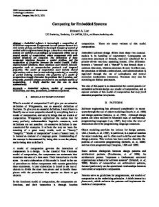
Figure 2: Graphical representation of the problem The problem can be expressed as a graph G = (V, E) shown in Figure 2. Vertex vi (1 ≤ i ≤ r + 1) represents the point where the first i phases have been executed. The M edges between vi and vi+1 (0 ≤ i ≤ r) represent different choices (which frequency to use) for phase i. Each choice is represented by a energy-time label, indicating the expected energy consumption and the worst-case running time for that phase. We also associate each path in the graph with a energy-time label where the energy of a path is defined as the sum of the energy of all edges over the path and the time of a path is defined as the sum of the time of all edges over the path. Therefore, the problem is reduced to finding a path from v0 to vr+1 such that the energy of the path is minimized while the time of the path is no greater than the deadline D. Notice that a path now can be summarized as a energytime label. A straightforward approach is to start from v0 and working all the way from left to right in an iterative manner. Each vertex vi is associated with a energy-time label set LABEL(i). Initially all label sets are empty except LABEL(0) which contains only one energy-time label (0, 0). The whole process consists of r + 1 iterations. In the ith iteration, we generate all paths from v0 to vi from LABEL(i − 1) and store them in LABEL(i). At the end, we just select the energy-time label with the minimum energy and with time no greater than D, from LABEL(r + 1), as the solution to the problem. Unfortunately, the size of LABEL(i) may suffer from exponential growth in this naive approach. To prevent this from happening, the key idea is to reduce and limit the size of LABEL(i) after each iteration by eliminating some of the energy-time labels in LABEL(i). There are two types of eliminations: one that does not affect the optimality of the solution and one that may affect optimality but still allows for performance guarantee.

5.2 Eliminations not Affecting Optimality There are three eliminations for LABEL(i) that do not affect the optimality of the solution: 1. For any energy-time label l in LABEL(i), if l.t + P i D, we eliminate this label. This is because even if the maximum frequency is used after this point, the deadline will still be missed; this implies label l will not lead to any feasible solution. f reqM

2. For the second elimination, we need to compare two energy-time labels. Definition 3. Let (e1 , t1 ) and (e2 , t2 ) be two energytime labels. We say that (e1 , t1 ) dominates (e2 , t2 )(denoted by (e2 , t2 ) ≺ (e1 , t1 )) if e1 ≤ e2 and t1 ≤ t2 . The dominance relation on a set of energy-time labels is clearly a partial ordering on the set. If (e2 , t2 ) ≺ (e1 , t1 ), this means (e2 , t2 ) will not lead to any solution better than the best solution which (e1 , t1 ) leads to. Therefore, we eliminate all energy-time labels that are dominated by some other energy-time label in the same label set. To facilitate this elimination, the energy-time labels in label sets are stored in decreasing order of the energy component, breaking ties with smaller time component coming ahead. Thus, this elimination can be performed using a linear scan of the label set. 3. For any energy-time label l in LABEL(i) surviving the previous two eliminations, one can use some heuristic to compute the upper bound of the optimal solution. One simple heuristic is to first find the optimal continuous frequency assuming that the task will run for the worst-case cycles, round it up and then compute the expected energy consumption assuming that this frequency is used from this point on. This energy plus l.e is an estimate of the upper bound of the optimal solution. Note that this operation can be done in constant time. We find the smallest estimated upper bound among all energy-time labels in LABEL(i), say U , then we do a linear scan of LABEL(i) to eliminate all energy-time labels whose energy is greater than U . With the eliminations above, the size of LABEL(i) would decrease substantially. Notice that at this point the optimal solution is guaranteed to be found. However, the running time of the algorithm still has no polynomial time bound guarantee. Inspired by the fully polynomial time approximation scheme (FPTAS) of the subset-sum problem [5], we obtain a FPTAS for our problem, presented next. The FPTAS, further reduces the size of LABEL(i).

5.3

Eliminations Affecting Optimality

The intuition for the FPTAS is that we need to further trim each LABEL(i) at the end of each iteration. A trimming parameter δ (0 < δ < 1) will be used to direct the

trimming. To trim a energy-time label set L by δ means to remove as many energy-time labels as possible, in such a way that if L′ is the result of trimming L, then for every energy-time label l that was removed from L, there is an energy-time label l′ < l still in L′ such that l.t > l′ .t ′ and l .e−l.e ≤ δ (or, equivalently, l.e ≤ l′ .e ≤ (1 + δ) · l.e). l.e This means that the energy difference between these labels is smaller than δ. Such a l′ can be thought of as “representing” l in the new energy-time label set L′ . Note that L′ ⊆ L. Let the performance guarantee be ǫ (0 < ǫ < 1), which means that the solution will be within a factor of 1 + ǫ of the optimal solution. After the first type of elimination described in Section 5.2, LABEL(i) is trimmed using a parameter δ = ln(1+ǫ) . The choice of δ shall be clear later in the proof of r+1 Theorem 2. The procedure TRIM (shown in Figure 3) performs the second type of elimination for label set L. Notice that at this point, the energy-time labels in label sets are stored in decreasing order on the energy component(or in increasing order on the time component).

1. 2. 3. 4. 5. 6. 7.

PROCEDURE TRIM(L = [l1 , l2 , . . . , l|L| ],δ) L′ := {l1 } last := l1 for i := 2 to |L| do if last.e > (1 + δ) · li .e then append li onto the end of L′ last := li return L′ END

Figure 3: TRIM(L,δ)

5.4 The PPACE Algorithm The PPACE algorithm is shown in Figure 4. For the sake of simplicity and clarity of presentation, the described algorithm is not the most efficient. We have a smarter implementation that makes the algorithm run faster but still has the same asymptotic behavior.

Considering the speed change overhead The problem formulation in (1)-(2) cannot capture the speed change overheads. This means that GRACE and PACE cannot deal with the speed change overheads simply because their solutions are based on the mathematical solution to (1)-(2). However, the PPACE algorithm can take into consideration the speed change overheads with a slight modification. Since the time penalty and energy penalty for a speed change depend on the speed before changing and the speed after changing [4], we only need to modify Line 7 of the PPACE algorithm such that if the chosen frequency for the current phase is different from that for the previous phase, we add the energy overhead to the energy component and add the time penalty to the time component of the newly generated energy-time label. In our experience with PPC750 embedded processors, we have observed (and the datasheets from the manufacture dictate) that the CPU will halt for a significant amount of time (10-50ms) each time the speed changes. The AMD PowerNow! processors have the same characteristic. For

ALGORITHM PPACE(ǫ) 1. for i := 1 to r + 1 do 2. LABEL(i) := φ 3. LABEL(0) = {(0, 0)} 4. for i := 1 to r + 1 do 5. for each label l ∈ LABEL(i − 1) do 6. for each available frequency f do 7. LABEL(i) := LABEL(i) ∪ (l + (si Fi e(f ), 8. remove all l ∈ LABEL(i) such that P

si )) f

sj

l.t + fiD reqM 9. remove all l ∈ LABEL(i) such that l ≺ l′ where l′ 6= l and l′ ∈ LABEL(i) 10. estimate the upper bound U , remove all l ∈ LABEL(i) such that l.e > U ) 11. LABEL(i) = TRIM(LABEL(i), ln(1+ǫ) r+1 12. return the label l ∈ LABEL(r + 1) with the minimum energy component END

Figure 4: PPACE algorithm these types of processors it is important to take into account the speed change overhead. However, for fair comparison with PACE and GRACE, we assume the speed change overhead is zero throughout the paper. Next, we show some results on the algorithm PPACE. First, notice that line 11 of the algorithm corresponds to the TRIM procedure, that is, the second type of eliminations (see Section 5.3). Let LABEL′ (i) (0 ≤ i ≤ r + 1) be the label set obtained if line 11 of the algorithm PPACE is omitted. Notice that LABEL(i) ⊆ LABEL′ (i) and the optimal solution is in LABEL′ (r + 1). By comparing LABEL(i) and LABEL′ (i), we have the following lemma: Lemma 1. For every energy-time label l′ ∈ LABEL′ (i), there exists a label l ∈ LABEL(i) such that l′ .e ≤ l.e ≤ (1 + δ)i · l′ .e and l′ .t ≥ l.t Lemma 1 shows how the error accumulates after each iteration when comparing label sets obtained with the second type of elimination and label sets obtained without the second type of elimination. For the details of the proof, see [18]. Theorem 2. PPACE is a fully polynomial-time approximation scheme, that is, the solution that PPACE returns is within a factor of 1 + ǫ of the optimal solution and the running time is polynomial in 1/ǫ. Proof. Let l∗ denote an optimal solution. Obviously l ∈ LABEL′ (r + 1). Then, by Lemma 1 there is a l ∈ LABEL(r + 1) such that ∗

l∗ .e ≤ l.e ≤ (1 + δ)r+1 · l∗ .e Since (1 + δ)r+1

=

µ

≤ =

eln(1+ǫ) 1+ǫ

1+

ln(1 + ǫ) r+1

¶r+1

then ∗

l.e ≤ (1 + ǫ) · l .e Therefore, the energy returned by PPACE is not greater than 1 + ǫ times the optimal solution. To show that its running time is polynomial in 1/ǫ, we first need to derive the upper bound on the size of LABEL(i). Let LABEL(i) = [l1 , l2 , . . . , lk ] after trimming. We observe that the energies of any two successive energy-time labels differ by a factor of more than (1 + δ) (otherwise, we have already eliminated it). In particular, l1 .e

> > .. . >

(1 + δ) · l2 .e (1 + δ)2 · l3 .e

(1 + δ)k−1 · lk .e P Moreover, l1 .e ≤ e(f reqM ) 0≤j≤i sj · Fj and lk .e ≥ P reqM ) e(f req1 ) 0≤j≤i sj · Fj . Let λ = e(f (i.e., the ratio e(f req1 ) of the energies when running with the highest and lowest frequencies), then (1 + δ)k−1