Apr 19, 2011 - Roberto Markarian 1, Sylvie Oliffson Kamphorst2 and Sônia Pinto-de-Carvalho2. Abstract. Inspired by the work of Pujals and Sambarino on ...
arXiv:1009.4187v2 [math.DS] 19 Apr 2011
Limit Sets of Convex non Elastic Billiards Roberto Markarian 1 , Sylvie Oliffson Kamphorst2 and Sˆonia Pinto-de-Carvalho2
Abstract Inspired by the work of Pujals and Sambarino on dominated splitting [17], we present billiards with a modified reflection law which constitute simple examples of dynamical systems with limit sets having dominated splitting and where the dynamics is a rational or irrational rotation.
1
Introduction
Let M be a Riemannian manifold and f : M → M ′ ⊂ M a diffeomorphism. An f -invariant set Λ has a dominated splitting if if its tangent bundle TΛ M = U ⊕ V , where U and V are non trivial invariant continuous subbundles such that, for constants C > 0 and 0 < γ < 1: kDf n |U (x) k kDf −n |V (f n (x)) k ≤ Cγ n , for all x ∈ Λ, n ≥ 0.
(1)
Clearly, any hyperbolic splitting is a dominated one. Some important consequences of this property on the dynamics were given by Pujals and Sambarino in [17]. A spectral decomposition theorem was obtained for C 2 compact surface diffeomorphisms [ having dominated splitting over the limit set L(f ) = (ω(x) ∪ α(x)) where ω(x) and α(x) are the x∈M
ω and α-limit sets of x, respectively:
Theorem (Pujals-Sambarino [17]): Let M be a compact 2-manifold and f : M → M ′ ⊂ M a C 2 -diffeomorphism. Assume that L(f ) has a dominated splitting. Then L(f ) can be decomposed into L(f ) = I ∪ R ∪ L˜ such that: 1. I is a set of periodic points with bounded periods contained in a disjoint union of finitely many normally hyperbolic periodic arcs or simple closed curves. 2. R is a finite union of normally hyperbolic periodic simple closed curves supporting an irrational rotation.
1
3. L˜ can be decomposed into a disjoint union of finitely many compact invariant and transitive sets (called basic sets). The periodic points are dense in L˜ and at most finitely many of them are non-hyperbolic periodic points. The (basic) sets above are the union of finitely many (nontrivial) homoclinic classes. Furthermore f |L˜ is expansive. Our purpose, in this work, is to construct simple examples of dynamical systems with attractors admitting a dominated splitting and where the dynamics is of type I or R. We will follow the ideas developed in [16] and [2]. In [16], non conservative billiards were introduced by a modification of the reflection rule and the existence of attractors was demonstrated for a wide class of dispersing and semi-dispersing billiards and of billiards with focusing components. In [2] models were studied numerically and different attractors, periodic and chaotic are presented. We concentrate on strictly convex billiard tables, with boundary formed by a unique sufficiently differentiable focusing component. They present structures like KAM stability islands and invariant rotational curves non homotopic to a point. We will investigate how, in the presence of non conservative perturbations, an invariant curve will give rise to an attractor. The maps we consider here are more general than the pinball billiards introduced in [16], as the perturbation of the angle is not necessarily biased to the normal direction. The contents of the present paper is outlined in four sections that follow this introduction. In section 2 we present the main tools needed to work with dominated splitting while section 3 deals with the basic properties of classical billiards on ovals. In section 4 we introduce our non elastic billiards. They are defined as a composition of a classical billiard followed by a change of the reflection angle, corresponding to a contraction in the vertical fibers of an invariant rotational curve. We will prove that under some differentiability hypotheses and some bounds on the contraction, there exists a compact strip in the phase space, such that the non elastic billiard map is a C 2 −diffeomorphism from that strip onto its image. Its limit set contains the invariant curve and has a dominated splitting. Moreover, the non elastic dynamics on the invariant curve is determined by its rotation number with respect to the original classical billiard map. This result will guide us to construct our examples of non elastic billiards on ovals with dominated splitting and attractors supporting a rational or an irrational rotation. They are presented in section 5, where we explore their properties theoretically and numerically. Our result (Theorem 1) could clearly be established in the more general setting of C 2 conservative twist maps. Once we have a C 2 invariant rotational curve and assuming the necessary bounds, everything would work likewise in the proof. The main problem is to build specific examples, other than the obvious twist integrable case (which corresponds to the circular billiard) or the oval billiards presented here, and check, for instance and at least numerically, the size of the basin of attraction.
2
2
Dominated Splitting, Cone Fields and Quadratic Forms
The existence of a dominated splitting follows from the existence of an eventually strictly invariant cone field and of an uniform control of expansions and/or contractions as showed in [21]. The criteria presented there in Proposition 4.1 can be translated, in dimension 2, into the operational lemma below. Let u, v : M 7→ T M be two vector fields such that u(x) = ux and v(x) = vx are linearly independent vectors in Tx M. They induce a nondegenerate quadratic form Q on T M by Qx (aux + bvx ) = ab and a cone field given at each x by C(x) = {w ∈ Tx M : Qx (w) > 0} ∪ {0} and whose boundaries, at each point, are given by C0 (x) = {w ∈ Tx M : Qx (w) = 0}. If the vector fields are continuous, the quadratic form and the cone field are also continuous. Given x ∈ M and a vector w = aux + bvx ∈ Tx M, let Dfx w = a1 uf (x) + b1 vf (x) ∈ Tf (x) M denote the image of w under the derivative Dfx . Then we have � � � � a a1 (2) = [Dfx ]U b b1 where [Dfx ]U is the matrix representation of the derivative at x, with the choice of {ux , vx } and {uf (x) , vf (x) } as bases of Tx M and Tf (x) M respectively. Lemma 1 Let Λ be a compact f -invariant subset of M. If there is a choice of vector fields u, v such that the entries of [Dfx ]U are strictly positive for every x ∈ Λ, then Λ has a dominated splitting. Proof: If the entries of [Dfx ]U are strictly positive for every x ∈ Λ then for every w = aux + bvx , x ∈ Λ, ab ≥ 0, a2 + b2 > 0 we have a1 b1 > 0 where Dfx w = a1 uf (x) + b1 vf (x) . This implies that for every x ∈ Λ Dfx (C(x) ∪ C0 ) ⊂ C(f (x)), i.e., C is strictly Df -invariant (f is strictly Q-separated). It follows from Proposition 4.1 in [21] that Λ has a dominated splitting. �
3
Classical Billiards on Ovals
Let Γ be an oval, i.e., a plane, simple, closed, C k , k ≥ 3, curve, with strictly positive curvature, parameterized counterclockwise by ϕ, the angle between the tangent vector and an horizontal axis. Let R(ϕ) be its radius of curvature at ϕ. The classical billiard problem on Γ consists of the free motion of a point particle inside Γ, making elastic reflections at the impacts with the boundary. The motion is then determined by the point of reflection at Γ and the direction of motion immediately after each reflection. They can be given by the parameter ϕ ∈ [0, 2π), that will locate the point of reflection and by the angle α ∈ (0, π) between the tangent vector and the outgoing trajectory, measured counterclockwise. 3
The classical billiard defines a map B from the open cylinder [0, 2π) × (0, π) into itself, which has some very well known properties (see, for instance, [10] and [11] for the properties of billiards and twist maps listed in this section). Denoting B(ϕ0 , α0 ) = (ϕ1 , α1 ), the derivative of B at (ϕ0 , α0 ) is � � 1 L − R0 sin α0 L DB(ϕ0 ,α0 ) = R1 sin α1 L − R0 sin α0 − R1 sin α1 L − R1 sin α1
(3)
where Ri = R(ϕi ) and L is the distance between Γ(ϕ0 ) and Γ(ϕ1 ). If Γ is C k , then B is a C k−1 -diffeomorphism. It preserves the measure dν = R(ϕ) sin α dαdϕ. It is reversible with respect to the reversing symmetry S(ϕ, α) = (ϕ, π − α), as S ◦ B = B −1 ◦ S, meaning that the phase space is symmetric with respect to the line α = π/2. Moreover, as Γ is an oval, B has the monotone Twist property with rotation interval (0, 1). For each ρ ∈ (0, 1) there exists a closed, invariant, minimal set Oρ ⊂ [0, 2π) × (0, π), which can be injectively projected on (0, 2π) and such that the induced dynamics preserves the order of [0, 2π) ∼ S 1 . This invariant set Oρ can be a periodic orbit, an Aubry Mather set or a rotational curve , i.e., a continuous closed curve which is the graph of a Lipschitz function. We will concentrate on billiards having an invariant rotational curve γ = graph(g), g : [0, 2π) 7→ (0, π) a Lipschitz function. In general, for a given boundary Γ, the set of rotation numbers ρ such that Oρ is an invariant rotational curve is nowhere dense in (0, 1), but nevertheless invariant rotational curves exist on a large class of classical oval billiards. For instance, the circular and the elliptical billiards have invariant rotational curves with any rotation number ρ. The billiard on a curve of constant width have the horizontal curve g(ϕ) ≡ π/2 as an invariant rotational curve with rotation number 1/2. But, apart from special examples like these, it is difficult to find billiards with invariant rotational curves of rational rotation number. In fact, having an invariant rotational curve with rational rotation number is not a generic property for billiards on ovals. The generic dynamics is to have, for each rational rotation number, a finite number of periodic orbits with this rotation number and at least one of them is hyperbolic, with transverse homoclinic orbits [7]. From the other side, having an invariant rotational curve with irrational rotation number is quite general. If the oval boundary Γ is C k , k ≥ 5 then Lazutkin Theorem guarantees a whole family of invariant rotational curves with diophantine ρ near the boundaries of the cylinder [0, 2π) × (0, π) ([13], [8]). And sufficiently small perturbations of the circular billiard present, in addition to the diophantine invariant rotational curves, given by the KAM theorem, uncountably many invariant rotational curves with liouvillian rotation number. For our purposes, we will need the curve γ, or equivalentely the function g, to be C 2 or more. This is the case of the circular, the elliptical and the constant width billiards, for instance, where the rotational invariant curves are, in fact, analytic. Also, the curves guaranteed by Lazutkin Theorem are as differentiable as the billiard map, so C 4 or more. But, as showed in [1], invariant rotational 4
curves can be just a little bit more regular than Lipschitz, and so we have to impose the existence of a C 2 rotational invariant curve as a condition to the billiards we will use. In the next paragraphs we present some bounds that will be necessary to prove our results. Let us assume that the invariant set Oρ is a closed curve γ= graph(g). As B|γ preserves the order of [0, 2π) ≈ S 1 then either g(ϕ) ≡ π/2 or there exist constants b and B such that 0 < b ≤ g(ϕ) ≤ B < π2 or π2 < B ≤ g(ϕ) ≤ b < π. The C 2 (or more) character of γ also implies that a tangent vector (1, g ′(ϕ0 )) is sent by DB(ϕ0 ,α0 ) on a tangent vector to γ at (ϕ1 , α1 ). The preservation of orientation implies that the first coordinate of DB(ϕ0 ,α0 ) (1, g ′(ϕ0 )) must be strictly positive. So R0 sin α0 >0 L This implies that g ′(ϕ) > −1 for every ϕ. As the billiard is reversible, the graph of g˜(ϕ) = π −g(ϕ) is also a rotational invariant curve and then g˜′ (ϕ) = −g ′ (ϕ) > −1 for every ϕ. So, for any C 2 invariant γ =graph(g), −1 < g ′ (ϕ) < 1. L[1 + g ′ (ϕ0 )] − R0 sin α0 > 0 and 1 + g ′ (ϕ0 ) >
To each invariant rotational curve γ is associated a caustic [18], a curve lying inside the billiard table and tangent to every segment of the billiard trajectory between two consecutive impacts. If (ϕ0 , α0 ) and so (ϕ1 , α1 ) belong to γ, then α0 = g(ϕ0), α1 = g(ϕ1 ) and we have R0 sin α0 R1 sin α1 + =L 1 + g ′ (ϕ0 ) 1 − g ′(ϕ1 )
(4)
where the two terms on the left hand side are strictly positive. The first one measures the distance to the tangency point (on the caustic) from the initial point Γ(ϕ0 ) and the second one, from the final point Γ(ϕ1 ) (see [15]).
4
Non Elastic Billiards
Let B(ϕ0 , α0 ) = (ϕ1 , α1 ) be a C 2 classical billiard map on an oval, with a C 2 invariant rotational curve γ0 , given by the graph of α = g(ϕ). A compact subset of the phase space [0, 2π) × (0, π) with non-empty interior and whose boundaries are two distinct rotational curves (not necessarily invariant nor graphs) will be called a compact strip. Let I ∈ IR be a closed interval containing 0. Given h : I → I, a C 2 strictly increasing contraction with h(0) = 0, we can define a non elastic billiard map P on a compact strip Σ containing γ0 by P (ϕ0 , α0 ) = (ϕ1 , α1 − h(α1 − g(ϕ1))) with Σ chosen such that if (ϕ, α) ∈ Σ then α − g(ϕ) ∈ I. P is the composition of a classical billiard followed by a change at the reflection angle, corresponding to a contraction in the vertical fibers of the invariant rotational curve γ0 . 5
Observe that h(t) ≡ 0 corresponds to the classical unperturbed billiard and that h(t) = t corresponds to a map that sends all the points in Σ onto the invariant curve (called slap billiard in [16]). The derivative of P is given by � �� � 1 L − R0 sin α0 L 1 0 DP(ϕ0 ,α0 ) = L − R0 sin α0 − R1 sin α1 L − R1 sin α1 R1 sin α1 h′1 g1′ 1 − h′1
(5)
where gi′ = g ′(ϕi ) and h′i = h′ (αi − g(ϕi )) Our main result is: Theorem 1 Given a classical oval billiard map B, with a C 2 invariant rotational curve γ0 = {(ϕ, g(ϕ))}, consider a compact strip Σ containing γ0 and a closed interval I ⊂ IR, such that α−g(ϕ) ∈ I if (ϕ, α) ∈ Σ. If h : I 7→ IR is a C 2 function satisfying h(0) = 0 and 0 ≤ 1−l < h′ (0) < 1 (with l depending only on γ0 ), then there exists a compact strip S ⊂ Σ such that the non elastic billiard map P defined by B, g and h is a C 2 -diffeomorphism from S onto P (S). Its limit set L(P ) contains γ0 and has a dominated splitting. Moreover, the non elastic perturbation does not change the dynamics on γ0 . Proof: The non elastic billiard P : Σ → P (Σ) ⊂ [0, 2π) × (0, π) is the composition of the C 2 classical billiard map B with the C 2 perturbation of the identity (ϕ, α) 7→ (ϕ, α) − (0, h(α − g(ϕ))), where h is a C 2 contraction. Then P is a C 2 diffeomorphism. Given δ > 0, let u(ϕ,α) = (1, g ′(ϕ) − δ) and v(ϕ,α) = (1, g ′(ϕ) + δ) be two linearly independent vector fields defining the cone field C(ϕ, α) and the associated quadratic form Q(ϕ,α) (as in section 2). Using the change of bases matrices, we have � � 1 δ(l0 − δL) + (1 − h′1 )(δl1 − l01 ) δ(l0 + δL) − (1 − h′1 )(δl1 + l01 ) [DP(ϕ0 ,α0 ) ]U = 2δR1 sin α1 δ(l0 − δL) − (1 − h′1 )(δl1 − l01 ) δ(l0 + δL) + (1 − h′1 )(δl1 + l01 ) (6) where l0 = L(1 + g0′ ) − R0 sin α0 , l1 = L(1 − g1′ ) − R1 sin α1 l01 = L(1 + g0′ )(1 − g1′ ) − (1 − g1′ )R0 sin α0 − (1 + g0′ )R1 sin α1 . Relation (4) implies that for every (ϕ0 , α0 ) and (ϕ1 , α1 ) on γ0 we have l01
1 − g1′ 1 + g0′ R1 sin α1 , l1 = R0 sin α0 . = 0 , l0 = 1 − g1′ 1 + g0′
The billiard boundary Γ is an oval and as it is compact there exist constants a and A and a width D such that 0 < a ≤ R(ϕ) ≤ A and 0 < L ≤ D. As the invariant curve is also compact, for 6
every (ϕ0 , α0 ) and (ϕ1 , α1 ) on γ0 , there exist constants c and C such that C ≥ l0 ≥ c > 0 and C ≥ l1 ≥ c > 0. So for points on γ0 there are constants 0 < l ≤ 1 and 0 < L such that l≤
l0 l1
and
0
0 such that δc(l − δL − (1 − h′ (0))) > 0. As P is a C 2 diffeomorphism and remembering that γ0 is compact, we can find a strip S ⊂ Σ, containing γ0 , where P is well defined and all the entries of [DP(ϕ0 ,α0 ) ]U are strictly positive. Then, by lemma 1, L(P ) ⊂ S has a dominated splitting and contains γ0 , since h(0) = 0. Moreover, P |γ0 = B|γ0 and the dynamics under P , on γ0 , is the same as under B. As γ0 and P are C 2 , for our billiard dynamics, γ0 is either a set of periodic points of same period linked by homo/heteroclinic arcs or supports a rational or an irrational rotation. � This result will guide us to construct examples of non elastic billiards on ovals with limit set having a dominated splitting and supporting a rational or an irrational rotation (pieces of type I or R of Pujals-Sambarino’s Theorem). This will be done in the next section. We will pay attention to the maximal possible size of the strip S and will try to see if there are other attractors on L(P ) than γ0 .
5 5.1
Examples The circle
The simplest example of a classical billiard with invariant rotational curves is the circular one. This billiard map is linear and is given by B(ϕ0 , α0 ) = (ϕ0 + 2α0 , α0 ). The phase space [0, 2π) × (0, π) is foliated by invariant horizontal curves and the dynamics on each one of them is simply a rotation of 2α0 . We pick one invariant curve γ0 , defined by α = g(ϕ) = β 0 . At γ0 , g ′ ≡ 0, Ri = R, the radius of the circle, and sin αi = sin β 0 , implying l0 = l1 and l = 1. Fix I, a closed interval with 0 ∈ I ⊂ (−β 0 , π − β 0 ) and h : I 7→ IR, any C 2 strictly increasing contraction such that h(0) = 0 and 0 < h′ (0) < 1. The non elastic billiard P is defined on the strip [0, 2π) × {I + β 0 } and is given by P (ϕ0 , α0 ) = (ϕ0 + 2α0 , α0 − h(α0 − β 0 )). By Theorem 1, there exists a compact strip S such that P |S is a C 2 diffeomorphism and L(P |S ) contains γ0 and has a dominated splitting. 7
Now, we choose β − and β + such that W = [0, 2π) × [β − , β + ] is the biggest horizontal straight strip contained in S. As each boundary γ± = {(ϕ, β ± )} is invariant under B, we have that P (W ) ⊂ W . The map P is a horizontal rotation followed by a vertical contraction. Denoting (ϕn , αn ) = P n (ϕ0 , α0 ), it is easy to see that αn → β 0 , as n → +∞ and so the horizontal circle γ0 is the unique attractor of P in W . Moreover, the restricted map P |γ0 is just a rotation of angle 2β 0 . If β 0 /π is rational, γ0 is a normally hyperbolic simple closed curve composed by periodic points of the same period. If β 0 /π is irrational γ0 is a normally hyperbolic closed curve supporting an irrational rotation. This yields an example of a diffeomorphism, defined on a strip W , whose limit set has dominated splitting and is composed by a unique piece of type I or R of Pujals-Sambarino’s Theorem. Clearly, the size of the strip W depends on the choice of the contraction h. Taking for instance h(x) = µx, with 0 < µ < 1, the non elastic billiard is given by P (ϕ0 , α0 ) = (ϕ0 + 2α0 , α0 −µ(α0 −β 0 )) and the basin of attraction of γ0 contains any straight strip W = [0, 2π) × [β − , β + ].
5.2
The ellipse
A similar example is given by the classical elliptical billiard. We consider an ellipse Γ with eccentricity √ 1 e and minor axis 1. Its radius of curvature R satisfies 1 − e2 ≤ R ≤ . The associated classical 1 − e2 billiard map is denoted by B : [0, 2π) × (0, π) 7→ [0, 2π) × (0, π). cos2 α − e2 cos2 ϕ is a first integral (see, 1 − e2 cos2 ϕ e2 for instance [3]) and [0, 2π) × (0, π) is foliated by the levels of F = F0 , with − 1−e 2 < F0 < 1. If 0 < F0 < 1, the level set consists of two invariant, analytic and symmetric rotational curves, the lower one contained in [0, 2π) × (0, π2 ) and the upper one in [0, 2π) × ( π2 , π). But, unlike the circular case, B has two elliptic islands of period 2, obstructing the rotational invariant curves to foliate the whole phase-space, as can be seen on Figure 1(left). It also has a hyperbolic 2-periodic orbit, with a saddle connection, corresponding to the level F0 = 0. This billiard system is integrable: the function F (ϕ, α) =
For a fixed 0 < F0 < 1 let γ0 be the lower invariant rotational curve inp F (ϕ, α) = F0 (the upper case is analogous). It is the graph of α = g(ϕ) given implicitly by cos α = F0 + (1 − F0 )e2 cos2 ϕ. p √ We have then that, for any (ϕ, α) ∈ γ0 , (1 − F0 )(1 − e2 ) ≤ sin α ≤ 1 − F0 . Differentiating twice with respect to ϕ we get (1 − F0 )e2 sin 2ϕ = g ′ (ϕ) sin 2α and 2(1 − F0 )e2 cos 2ϕ = 2g ′(ϕ) cos 2α + g ′′(ϕ) sin 2α. The extremal points of g ′ must satisfy tan 2ϕ = tan 2α which implies max{g ′(ϕ)} = (1 − F0 )e2 = − min{g ′ (ϕ)}. We can then take �2 � l0 (1 + g0′ )2 R1 sin α1 1 − (1 − F0 )e2 2 2 = (7) ≤ l = (1 − e ) ′ 2 2 1 + (1 − F0 )e (1 − g1 ) R0 sin α0 l1 The associated non elastic billiard map is given by P (ϕ0, α0 ) = (ϕ1 , α1 − h(α1 − g(ϕ1)) where the contraction h : I 7→ IR is an arbitrary C 2 function satisfying h(0) = 0 and 0 < 1 − l ≤ h′ (0), and I 8
is a closed interval containing 0. Then, by Theorem 1, there exists a compact strip S, containing γ0 , such that P |S is a C 2 diffeomorphism, L(P |S ) has a dominated splitting and contains γ0 . Let F± be two constants of motion satisfying 1 > F− > F0 > F+ > 0, and γ± =graph(g± ) be the lowest invariant rotational curves associated to F± , respectively. We also suppose that W = {(ϕ, α), g−(ϕ) ≤ α ≤ g+ (ϕ)} ⊂ S is the biggest strip of this type contained on S. As γ± are invariant under B we have P (W ) ⊂ W . For (ϕ0 , α0 ) ∈ W , we denote (ϕn , αn ) = P n (ϕ0 , α0 ). Let us suppose, for instance, that F (ϕ0 , α0 ) > F0 , the other case being analogous. As P is a translation on a B-invariant rotational curve followed by a contraction on the vertical direction toward γ0 , then F (ϕn , αn ) → F0 and γ0 is the ω-limit of any (ϕ0 , α0 ) ∈ W . As in the circular case, γ0 is the unique attractor of P |W . Using action-angle variables, Chang and Friedberg [5] have shown how to decide if the rotation number associated to the level F0 = F (ϕ0 , α0 ) of a given initial condition (ϕ0 , α0 ), is rational or irrational and then determine the dynamics on each level curve. As P |γ0 = B|γ0 , this allows us to choose F0 in order to have, as the unique attractor, a normally hyperbolic closed curve supporting an irrational rotation or a normally hyperbolic closed curve composed by periodic points of same period. Although theoretically promising as a result, depending on the choice of γ0 and h, the strip W can be very thin. In particular it will never contain points of the elliptical islands. In trying to go beyond the theoretical predictions and find examples of non elastic elliptical billiards defined on a bigger part of the phase space, we shall remember that weak contractions will never destroy the rotation carried by the linear ellipticity of the 2-periodic orbit. So we can not expect the associated non elastic billiard to be defined on a strip containing the islands. However, it is an interesting question whether this can be achieved by taking a sufficiently strong contraction. We present some numerical simulations where this can be done. We choose an ellipse with e = 0.35 and fix the invariant curve γ0 at F0 = 0.25. Our choices of the eccentricity and γ0 are rather arbitrary. Figure 1 (left) below diplays the phase space of the classical elliptical billiard. The invariant curve γ0 is enhanced. The horizontal axis corresponds to ϕ ∈ [0, 2π) and the vertical to α ∈ (0, π), the left bottom corner being the origin. We consider linear perturbations h(x) = µx, with 0 < µ < 1. µ = 0 implies that there is no perturbation (classical billiard) and µ = 1 implies that all the points in the phase space land on the invariant curve after one iteration (slap billiard). The non elastic billiard P (ϕ0 , α0 ) = (ϕ1 , α1 − µ(α1 − g(ϕ1 ))) is a C 2 diffeomorphism on any compact strip contained on [0, 2π) × (0, π). Calculating l by formula (7) we get that if µ > 1 − l ≈ 0.47 there is a strip W such that γ0 is the unique attractor of P on W and has a dominated splitting. Figure 1 (right) illustrates the basin of attraction of the curve γ0 for µ = 0.5: black points correspond to initial conditions which approach γ0 under iteration. This simulation thus indicates that the basin of attraction of γ0 is the whole phase space, ie, that W can be any compact strip contained in [0, 2π) × (0, π) and γ0 is the unique attractor of P . Note that, as we have mentioned before, either γ0 is composed of periodic points of same period or supports an irrational rotation.
9
Figure 1: Classical and non elastic elliptical billiards
5.3
Non integrable billiards
There are no other known C 2 ovals such that the classical billiard map is integrable, other than the circle and the ellipse. But it is well known that there are oval billiards with C 2 invariant rotational curves. Taking a sufficiently differentiable, non integrable, classical oval billiard map B with a C 2 invariant rotational curve γ0 =graph(g) we can, as before, take a contraction h satisfying the hypothesis of Theorem 1 and define a non elastic billiard map P . Then there exists a strip S on which P is a C 2 diffeomorphism on S, L(P ) contains γ0 and has a dominated splitting. Depending on the rotation number of γ0 we can have, as in the previous examples, a normally hyperbolic closed curve supporting an irrational rotation or a normally hyperbolic closed curve composed by periodic points of same period. But we can no longer guarantee that the only attractor of P is γ0 . 5.3.1
Invariant straight line
In order to explore numerically what happens in those more general cases, we have to pick a concrete example. Although in any example one can prove the existence of whole families of invariant curves, it is almost impossible for any fixed curve, to write down the function g for which it is the graph. In general this can only be achieved in very specific examples as, for instance, the constant width curves, where g(ϕ) = π/2. We will deal with a much richer example, given by symmetric perturbations of the circle. Let Γn be the oval parameterized by the angle ϕ and which radius of curvature is of the form R(ϕ) = 1 + a cos nϕ, |a| < 1 and n ≥ 4. Tabachnikov (Section 2.11, [18]) showed that its associated classical billiard map have an invariant straight line given by g(ϕ) = β0 if β0 satisfies n tan β0 = tan nβ0 . It is not difficult to show that the dynamics on γ0 is an irrational rotation [9]. 10
√ For n = 6, β0 = tan 7 + 4 21/3 ≈ 0.41π satisfies this condition and the line γ0 given by α = g(ϕ) = β0 is invariant. Figure 2 displays the billiard table and the corresponding phase space of Γ6 defined by R(ϕ) = 1 + 0.01 cos 6ϕ. As in the previous section, the horizontal axis corresponds to ϕ ∈ [0, 2π) and the vertical to α ∈ (0, π), the left bottom corner being the origin. Note the invariant straight line γ0 . −1
q
Figure 2: Billiard table and classical phase space for Γ6 As in the other numerical examples, we consider linear perturbations h(x) = µx, 0 < µ < 1. On γ0 , min R(ϕ) 0.99 = 1.01 . Then, if µ > 1−l ≈ 0.02, we have l0 = R1 sin β0 and l1 = R0 sin β0 and we can take l = max R(ϕ) 2 there exists a strip S on which P is a C diffeomorphism, L(P ) contains γ0 and has a dominated splitting. Figure 3 illustrates the basin of attraction of γ0 for µ = 0.1, 0.35, 0.37 and 0.4: black points correspond to initial conditions which approach γ0 under iteration. The white tadpoles correspond to points attracted to the 6-periodic orbits, linearly elliptic for the original classical billiard. We observe that as the contraction factor µ is increased, the basin of attraction of γ0 grows until it eventually occupies the whole phase space. Thus, for strong contractions, we may have P defined on any compact strip S and having γ0 as its unique attractor.
5.4
An example that is not one
Any strictly convex classical billiard map is a monotone twist map with rotation interval (0, 1). To each ρ ∈ (0, 1) is associated a set Oρ . If ρ is irrational, Oρ is either a rotational invariant curve or an Aubry-Mather set. An Aubry Mather set is a closed, invariant, minimal set, projecting injectively on a Cantor set of S 1 ∼ [0, 2π) and such that the dynamics preserves the order of S 1 . It is contained in 11
a non invariant graph of a continuous piecewise linear Lipschitz function α = g(ϕ) (see, for instance [10], Section 13.2). Let us take a classical billiard map B with two rotational invariant curves γ− and γ+ and an AubryMather set A contained in the strip bounded by γ− and γ+ and a perturbation h on this strip. The non elastic billiard map can be then defined as before, as P (ϕ0 , α0 ) = (ϕ1 , α1 − h(α1 − g(ϕ1)), where (ϕ1 , α1 ) = B(ϕ0 , α0 ). As h is a contraction, the limit set of P will contain the Aubry-Mather set A. However, we must remark that P is not C 2 because g is not even a differentiable function. Then, we can not apply Pujal-Sambarino’s theorem. Acknowledgment. We thank M´ario Jorge Dias Carneiro for his precious ideas. We thank the Brazilian agencies FAPEMIG and CNPq for financial support.
References [1] Arnaud M C 2009 Publ. Math. Inst. Hautes Etudes Sci 109 1–17 [2] Arroyo A, Markarian R and Sanders D P 2009 Nonlinearity 22 1499–1522 [3] Berry M 1981 Eur. J. Phys. 2 91–102 [4] Birkhoff G D 1932 Bull. SMF 60 1–26 [5] Chang S J and Friedberg R 1988 J. Math. Phys. 29 1537–1550 [6] Chernov N I and Markarian R 2006 Chaotic Billiards. Mathematical Surveys and Monographs 127 . American Mathematical Society. [7] Dias Carneiro M J, Kamphorst S O and Pinto-de-Carvalho S 2007 Nonlinearity 20 24532462 [8] R.Douady: Applications du th´eor`eme des tores invariants. Th`ese de 3`eme Cycle, Univ. Paris VII, 1982. [9] Ferreira, G.: Billiards maps with invariant straight lines and curves. of Abstracts of The Second International Conference BILLIARDS’2011, http://www.rc.unesp.br/igce/demac/billiards11/
Book 2011,
[10] Katok A and Hasselblatt B 1997 Introduction to the Modern Theory of Dynamical Systems. (Cambridge Univ. Press) [11] Katok, A., Hasselblatt, B.: Principal Structures, in Handbook of Dynamical Systems, vol 1A, ed. Hasselblat, Katok, North-Holland, 2002. [12] Knill O 1998 Elem. Math. 53 89–106
12
[13] Lazutkin V F 1973 Math. USSR Izvestija 7 185–214 [14] Markarian R. 1988 Comm. Math. Phys. 118 8797. [15] Markarian R, Kamphorst S O and Pinto-de-Carvalho S 1996 Comm. Math. Phys. 174 661–679 [16] Markarian R, Pujals E R, Sambarino M: Pinball billiards with dominated splitting, ETDS , 30, 1757-1786, 2009. Erg. Th. Dyn. Sys. [17] Pujals E R and Sambarino M 2009 Ann. Math. 169 675–740 [18] Tabachnikov S 1995 Billiards (Paris: Soci´et´e Math´ematique de France) [19] Wojtkowski M 1985 Ergod. Th. & Dynam. Sys. 5 145–161. [20] Wojtkowski M 1986 Commun. Math. Phys. 105, 391414. [21] Wojtkowski M 2001 Smooth Ergodic Theory and Its Applications, Proc. Symp. Pure Math. vol 69 (AMS) 499–521
13
Figure 3: Γ6 : the basin of attraction of γ0 for µ = 0.1, 0.35, 0.37 and 0.4
14