I. J. Computer Network and Information Security, 2017, 2, 1-11 Published Online February 2017 in MECS (http://www.mecs-press.org/) DOI: 10.5815/ijcnis.2017.02.01
Limitations of Passively Mapping Logical Network Topologies Ayodeji J. Akande School of Electrical Engineering and Computer Science, Queensland University of Technology, GPO Box 2434, Brisbane, QLD 4001 Queensland, Australia E-mail:
[email protected]
Colin Fidge and Ernest Foo School of Electrical Engineering and Computer Science, Queensland University of Technology, GPO Box 2434, Brisbane, QLD 4001 Queensland, Australia E-mail: {c.fidge, e.foo}@qut.edu.au
Abstract—Understanding logical network connectivity is essential in network topology mapping especially in a fast growing network where knowing what is happening on the network is critical for security purposes and where knowing how network resources are being used is highly important. Mapping logical communication topology is important for network auditing, network maintenance and governance, network optimization, and network security. However, the process of capturing network traffic to generate the logical network topology may have a great influence on the operation of the network. In hierarchically structured networks such as control systems, typical active network mapping techniques are not employable as they can affect time-sensitive cyberphysical processes, hence, passive network mapping is required. Though passive network mapping does not modify or disrupt existing traffic, current passive mapping techniques ignore many practical issues when used to generate logical communication topologies. In this paper, we present a methodology which compares topologies from an idealized mapping process with what is actually achievable using passive network mapping and identify some of the factors that can cause inaccuracies in logical maps derived from passively monitored network traffic. We illustrate these factors using a case study involving a hierarchical control network. Index Terms—Network logical topology, network modeling and mapping, network observability, network monitoring, network traffic analysis, network graph.
I. INTRODUCTION In practice, an existing physical network topology is not always the same as the original documented version of the physical network topology developed for the network. There is a need for an up-to-date knowledge of the network topology. Network topology mapping is becoming increasingly important especially in fast growing networks where the understanding of what is happening in the network is essential. Network traffic Copyright © 2017 MECS
analysis is a fundamental tool used in constructing network topologies. Information such as the source address, destination address and communication protocols obtainable from observed network data packets, is a prerequisite for network topology mapping [21]. Network topology mapping is an essential technique used by network administrators and system analyst for network maintenance and governance, network optimization, network security and auditing. In traditional IT communication networks, active mapping techniques are used but in time-sensitive control network, active mapping may affect negatively the network‘s operation, hence, passive network mapping is required. Passive monitoring involves observing network traffic that is already on the network without traffic modification or disruption of the network‘s performance. In comparison, active monitoring techniques such as IP ping, traceroute and Network mapper (Nmap) can cause critical infrastructure equipment to stop working or cause delays to a time critical network due to the addition of overhead on the monitored communication paths. Passive monitoring uses tools such as mirror or span ports and network taps designed to unintrusively capture network traffic. Evaluation of network traffic entails analyzing source and destination communication, that is, the data flow between network devices to identify the ―logical topology‖ of the network. The logical topology represents how the devices communicate with one another. Hosmer [14] developed an open source program known as Python Passive Network Mapping (P2NMAP) to passively monitor a network to identify network devices and to identify unusual behaviors in the network. Hosmer [14] stated that depending upon how long the network was monitored, every node with an IP address on the network can be identified and how they are connected with each other on the network. Other information that can be deduced using Hosmer‘s approach includes details of where and what devices have communicated, and at what time the communication was made. Though, topology mapping using passive monitoring was practically addressed by Hosmer‘s work,
I.J. Computer Network and Information Security, 2017, 2, 1-11
2
Limitations of Passively Mapping Logical Network Topologies
the limitations of passive monitoring in topology discovery was not discussed. The contribution of our paper is to identify the challenging issues in the use of passive monitoring for topology mapping. To do this, we present our experimental methodology which involves deriving an expected logical topology from the documented physical network topology, generating the observed logical topology from passively captured network traffic and then comparing the two logical topologies to identify the differences between what is observable in theory and in practice. Our results indicated that the expected topologies and the observed topologies did not completely align. We analyzed the results to determine why and found several reasons including inactive devices, broadcast messages with no destination address and newly introduced devices. We concentrated on available information from passively captured traffic, which includes layer 2 information (MAC Addresses) and layer 3 information (IP addresses) in the network packet header. Our contribution gives an insight into the extent to which topology observability is possible using passive network monitoring. In order to demonstrate the methodology of passively mapping a critical infrastructure network, a Supervisory Control and Data Acquisition (SCADA) network was used as a case study. A SCADA network is considered as a representative example of a critical infrastructure network due to the network‘s hierarchical structure, its wide variety of components, its use of subnets and its distinct traffic pattern and its use in remotely controlling industrial processes. The rest of the paper is as follows: Section 2 is the related work. Discussed in Section 3 are principles involved in passive network traffic monitoring and topology generation. Section 4 is our experimental methodology, while in Section 5 is a case study. Section 6 presents our comparative analysis results. Section 7 concludes our work and highlights our future research directions.
II. RELATED WORK Numerous vendors have developed commercial proprietary management tools and protocols useful for automatic topology discovery. These tools are mostly Simple Network Management Protocol (SNMP) based. Examples of such tools include HP‘s OpenView, IBM‘s Trivoli, AdvertNet OpManager, Actualit‘s Optimal Surveyor, Dartmouth Intermapper [5, 20] and the Cisco Prime Network is useful in network topology discovery [9]. Also in the research community, efforts have been made in the area of network topology discovery in Internet structure and Ethernet networks mainly using SNMP [4, 18, 20], ping/broadcast ping, zone transfer from DNS server and skitter [1, 11, 15]. Algorithms based on SNMP [5, 16, 17, 19], have been developed to obtain topology information such as IP addresses from targeted devices‘ SNMP Management Information Bases (MIBs) which store object identifier (OID) numbers and network parameters in a tree Copyright © 2017 MECS
formatted hierarchy. Breitbart et al. [5] presented an algorithmic solution, which was developed to solve the problem of physical topology discovery in heterogeneous IP networks. Their algorithmic solution was based on SNMP, which uses information obtained from address forwarding tables containing Medium Access Control (MAC) addresses that are reachable from each device interface. Though the SNMP based algorithm generated remarkable results, the process of fetching packet information from the network is inefficient especially in modern standard IT networks and critical infrastructure networks. The algorithms depend on active probing mechanisms such as the ICMP ping mechanism and traceroute to adequately populate the SNMP MIBs and obtain complete network information [5]. The process of obtaining the topology information introduces additional overhead to the monitored path. Other weak- nesses in the use of SNMP base algorithms include access restrictions to some device SNMP MIBs and some devices do not support SNMP [10]. The use of active techniques, especially in control systems, can cause network devices to shutdown, lockup or failed, hence, the need for passive monitoring. Passive monitoring has been used in analyzing traffic flow and topology discovery by several researchers [6, 7, 12, 2]. In a paper by Castillo et al. [7], the observability problem in traffic network models was explored. In addressing the observability problems, two algebraic methods were proposed. The first proposal was the one global approach, which is based on null-spaces. The second proposal was one step-by-step procedure that allows the update of information of each item of OriginDestination (OD) pair or link flow once it is available. The proposed methods by Castillo et al. are useful in inferring information of OD-pair or link flows. Similarly, Hosmer [14] developed a tool to passively monitor network traffic and extract topology information from the captured packets. P2NMAP passively captures packets flowing to and from TCP Port 443 and extracts key data such as serverIP, ClientIP and serverPort fields from packets traversing the network being monitored. Although, Hosmer [14] described a network mapping algorithm using Python to generate a list of sourcedestination pairs from passively observed traffic, Hosmer failed to address the extent to which the generated list can be used to develop logical communication topology to express the physical network topology and also failed to address the accuracy of passive monitoring in generating an accurate logical topology of a network. Though passive monitoring aims to monitor network traffic without affecting the network latency, our major concern is with the accuracy of techniques for generating network topology map from passively monitored network traffic. In our research we have identified some factors that affect the accuracy of logical maps derived from passively monitored network traffic in practice and in this paper we investigate these factors.
I.J. Computer Network and Information Security, 2017, 2, 1-11
Limitations of Passively Mapping Logical Network Topologies
III. NETWORK TOPOLOGY GENERATION Network monitoring is an essential and standard tool for learning what is happening in a network. The technique entails capturing network packet traffic and analyzing it. The general principles involved in passive topology generation from network traffic monitoring and topology generation are discussed in this section with a focus on mapping the logical communications topology of a network. We define a logical network topology as a topology that represents the end-to-end communication flow between devices on the network. Though the physical layout of the devices on the network is represented by its physical topology, the logical topology reveals what communication actually occurs in the network. Cecil [8] described two types of network topology monitoring, which are non-router based techniques. These are active network topology monitoring and passive network topology monitoring. Active network topology monitoring techniques such as ping and traceroute, involve probing targeted devices by sending commands to obtain traffic information. However, active probing requires prior knowledge of the identities and type of existing network devices and more importantly, disrupts the normal flow of network traffic, which is unacceptable in a time-sensitive control system. Passive network topology monitoring, unlike active monitoring, does not involve injecting or sending any commands to probe specific devices. In passive network topology monitoring, traffic flowing through an observation point is passively captured without modifying the traffic that is already in the network. Also, in passive network topology monitoring, the observer may be invisible to its neighboring devices, that is, the observing device may not generate any messages but only observe traffic flowing through it. Using passive network topology monitoring, a logical network topology can be generated from the captured network traffic. In this paper, the generated topology is referred to as observed logical network topology. However, to verify the accuracy of this observed logical network topology, generated from captured network traffic via a passive observer, we need to calculate what the observer is expected to see under ideal circumstances. This derived logical topology is referred to as the expected logical topology. Described below are our assumptions used for calculating what a passive observer is expected to see given a known physical network layout. A.
Assumptions
Though our research goal is to generate a logical network topology from passively monitored traffic, first we need to understand what part of a network‘s logical communication topology we would expect to be visible to ‗observers‘ who capture data traffic at different locations. In practice, it is reasonable to assume that messages (usually!) follow a shortest path between their source and destination (keeping in mind that there may be several equally-long shortest paths). In this case, the observable Copyright © 2017 MECS
3
logical topology can be considered as a directed graph and will include a connection from a source to a destination iff all shortest paths between the nodes in the digraph include an observer. We make some major assumptions. We assume the set of nodes is partitioned into two groups, ‗visible‘ and ‗invisible‘. Visible nodes are those that may be the original source or final destination of messages. Visible nodes are thus ―noisy‖ and may appear in the observable logical topology. In practice, visible nodes are typically computing devices or routers, each with a unique address. Invisible nodes are those that neither generate new messages nor act as the final destination for a message; instead they forward messages from one of their incoming edges to one or more outgoing edges. These intermediate nodes will not appear in the logical topology. In practice, invisible nodes are usually simple switching devices, needed to move packets through the physical network. We make a further assumption that we observe the network for long enough for every possible sourcedestination pair of ‗active‘ nodes to communicate via at least one message. This assumption maximizes how much of the logical graph can be observed. Also, we assume a distinguished subset of the nodes additionally serve as ‗observers‘ of network traffic. Observer nodes record the details of messages passing through them and are the way in which we can see network activity. Observer nodes may be either visible or invisible. In the case of a visible observer, we assume it records all messages it generates or receives, as well as messages it merely forwards. In practice, a visible observer will usually be any device with a mirror port to capture data packets sent, received or forwarded, while an invisible observer will be an in-line tap which silently copies passing data packets, but never generates or receives packets of its own. For our purposes the only data that needs to be recorded by an observer are the ―from‖ and ―to‖ fields in the packet headers. Finally, we assume that if source and destination addresses are observed in a packet, we presume the source and destination both exist. In practice, not every addressed node is a legitimate node. Under these assumptions, in the next section, we consider how much of the logical communications topology can be gleaned from the messages recorded by observers at particular locations in a physical network. The answer depends on the way in which active nodes generate messages, the routing of messages through the network and the location of observer. Before going into details of our experimental approach, we need to define what an observer is expected to see if passively observing traffic in the network. B.
Observability definition
We use standard set-theoretic definitions for directed graphs and paths through such graphs. Let a directed graph or digraph, G = (V, E), be a tuple consisting of a set of vertices V and asset of edges E ⊆ V × V. Let an edge, (v1, v2) ∈ E, be an ordered pair denoting a
I.J. Computer Network and Information Security, 2017, 2, 1-11
4
Limitations of Passively Mapping Logical Network Topologies
unidirectional link between a source vertex v 1 ∈ V and a destination vertex v2 ∈ V. We can represent the graph as an adjacency matrix [13] as shown in equation (1):
(1) n Let a path, ⟨v1, v2, . . . vn⟩ ∈ V , of length n through graph G = (V, E) be an ordered set (or ‗sequence‘) of vertices vi ∈ V such that, for all vi where1 ≤ i ≤ n, there exists an edge (vi, vi+1) ∈ E in graph G. As a special case, let a simple path, ⟨v1, v2, . . . vn⟩, of length n through graph G be a path in which there are no duplicated vertices in the sequence, i.e., a path such that vi≠vj for all i,j ∈ {1,...,n} where i≠j. We assume the existence of standard functions on digraphs for finding paths between vertices and calculating the graph‘s transitive closure. Given a digraph G = (V, E), a source vertex α ∈ V, and a destination vertex ω ∈ V, let the set of all paths between these vertices be all paths of the form {α, v2...vn−1, ω} through graph G, i.e., those paths through G such that the first vertex is α and the last vertex is ω. This set will be empty if no path from α to ω exists through G. We denote the function that returns the set of all paths from α to ω through graph G by pt (α, ω, G). Given a digraph G = (V, E), a source vertex α ∈ V, and a destination vertex ω ∈ V, let the set of all shortest paths between these vertices be all paths {α, v2...vn−1, ω} of length n through graph G such that there does not exist a path {α, x2...xm−1, ω} of length m through G where m < n, i.e., all paths from α to ω for which there is no shorter path between these vertices. This set will be empty if no path from α to ω exists through G, and it may contain multiple values if several shortest paths of the same length exist between α and ω. Note that our definition of shortest paths is based on the number of hops between the source and destination; we assume all edges have equal weight. We denote the set of all shortest paths from α to ω through graph G by sh (α, ω, G). Finally, given a digraph G = (V, E), let its transitive closure be a digraph H = (V, F) such that, for all pairs of edges (α, ω) ∈ V × V, edge (α, ω) appears in iff there exists a path between α and ω through G. We denote the transitive closure of graph G by tr (G). Definition: Network observability, we assume that packets will be sent from their source to their destination via the shortest path, so will be seen only by observers on that path. However, keeping in mind that there may not be a unique shortest path between two nodes, we require that there is an observer on every shortest path between the source and destination, to ensure that messages routed via shortest paths can‘t avoid being seen. We also assume that nodes do not send messages to themselves. Given a physical topology G, a set O of observer vertices and a set I of invisible vertices, we can then Copyright © 2017 MECS
define the logical topology we would expect to observe. Let W = V \ I be the set of all vertices that may appear in the logical communications topology. Then the logical topology observable in such a network is H = (W, F), where F ⊆ W × W, such that for all potential sourcedestination pairs (α, ω) ∈ tr (G), edge (α, ω) appears in F iff (i) α≠ω, and (ii) α ∈ W, and (iii) ω ∈ W; and either (iv) α ∈ O, or (v) ω ∈ O, or (vi) for all shortest paths P ∈ sh(α, ω, G) there exists an observer o ∈ O such that o ∈ P. C.
Example
We present a simple example, which illustrates the difference between the ―physical network‖ topology and the ―expected‖ logical topology observable from captured net- work traffic. In Fig. 1 is the physical network topology of network, which comprises four devices A, B, C and D where C is the observer.
Fig.1. Physical Network Topology
The physical topology in Fig. 1 is modeled and translated into an adjacency matrix as shown in Fig. 2 below. Fig. 3 is the expected logical topology observable from the network shown in Fig. 1 according to our definition. The difference between the two graphs is that in Fig. 3, all nodes were seen but not all connections are shown. In Fig. 3, this is no path between B and D because there is a shorter path directly from B to D that the observer C cannot see.
Fig.2. Matrix Representation of Physical Network Communication
Fig.3. Expected Logical Topology as Observed by C
I.J. Computer Network and Information Security, 2017, 2, 1-11
Limitations of Passively Mapping Logical Network Topologies
IV. THE EXPERIMENTAL METHODOLOGY In this section, we present our experimental approach, which compares the topologies, generated from passively monitored traffic with the idealized topologies derived from the network model assuming ideal circumstances. Fig. 4 is the overview architecture of our approach, which consists of three parts. The first part is the box on left labeled the ‗expected topology definition‘ where we define what an observer is expected to observe under an ideal circumstance to produce an expected topology. The second part is ‗network traffic mapping‘ which involves the observation of a real network by passively monitoring the network traffic flowing through the selected observers and generating an actual topology. The final process is ‗topology comparison‘ where we compare the generated topologies to check for differences. The entire process was automated using a library of Python scripts. A.
Expected Topology Derivation
a)
Network modeling from physical network
Given the physical network‘s design, we represent each interface on each physical device as a node and the edges between them represent communications links. The connectivity between nodes is represented as an adjacency matrix using 1 to symbolize nodes communicating with each other and 0 to symbolize no communication in our representation in Fig. 2. A subset of the nodes is then selected as ―observers‖. Similarly some nodes are selected as ―in- visible‖, as per the assumed physical topology. Observer vertices are those network locations at which we assume data traffic is being monitored. Typically they denote net- work devices such as in-line taps or mirror ports that ‗capture‘ copies of passing data traffic for analysis. The location of an observer limits what is seen while passively monitoring traffic. b)
referred to earlier. The steps for calculating the network observability to the observers given the physical topology are as follows: Initialize an empty adjacency matrix Add connections between each observer and all other nodes (under our assumption that all nodes communicate with one another) For each connection in the physical topology‘s transitive closure, add this link to the matrix iff the source and destination nodes are different and all shortest paths between the source and destination contain an observer. Remove all ‗invisible‘ nodes (and their connections) from the matrix. We implemented this calculation as a simple Python program and used an off-the-shelf drawing package to visualize the resulting graphs. B.
The expected topology is derived from the original physical network design. It presents the anticipated observable logical communication and is derived based on what the observers can see from their location on the network given our shortest path assumption. This section presents process for deriving the expected topology as indicated on the left hand side of our methodology in Fig. 4. Given that the physical network design is known, below are the steps to derive the expected topology.
5
Network Traffic Mapping
Mapping a network‘s logical topology gives us knowledge of the communication pattern of the network. To achieve this, network traffic analysis is required. In this section, we present our network traffic mapping technique, which is part of our experimental methodology as indicated on the right hand side of Fig. 4. Traffic mapping involves the extraction of source and destination addresses from the captured network packets. The mapping process used in this paper to generate a logical network topology from passively captured traffic is via four processes: identification of observers; network capture; data extraction and topology generation. Network physical topology Selection of observers
Network Modelling
Network Capture
Derivation of anticipated/expected logical topology
Data Extraction
Expected topology definition
Generation of actual logical topology
Derivation of expected logical topology
The second procedure is the observability analysis, which is required to understand what part of a network‘s logical communication topology is visible to ‗observers‘ who passively monitor data traffic at different locations. We calculate the potential observability based on a reachability analysis of the network‘s physical topology using the observability definition described in Section 3.2. In particular, we analyze what should be seen given the assumptions about observer locations, device visibility/addressability, and message-routing protocols Copyright © 2017 MECS
Network Traffic Mapping
Comparison of topologies Fig.4. Implementation Architecture of the Experimental Methodology
i.
Identification of observer(s)
This first step involves identifying the location of a non-empty set of devices to serve as observers to passively monitor the network traffic flowing. Passive monitoring provides detailed topology information about
I.J. Computer Network and Information Security, 2017, 2, 1-11
6
Limitations of Passively Mapping Logical Network Topologies
one point on the network that is being monitored. The location of an observer limits what is seen while passively monitoring traffic. Monitoring a single device or point in a network may not be adequate for logical topology discovery of the entire network depending on how large the network is and its traffic routing. Monitoring traffic at various locations on the network and adding all the captured traffic into one file for processing may be required to obtain substantial information for generating a full logical topology. ii.
V. CASE STUDY A SCADA network was developed as shown in Fig. 6 in a simulated environment. Supervisory Control And Capture network traffic, initialise source-destination pair list
More packets to process?
Network capture
This step requires capturing network traffic at the selected observer to obtain the packet information needed to generate a logical topology of the network. Network traffic can be passively monitored using a network tap or the use of built-in capabilities on switches such as port mirroring [8]. The captured traffic is then converted to a csv file and processed off-line. iii.
iv.
Topology generation
The last step is the generation of the logical topology from the list of source-destination pairs into an adjacency matrix representation and then generating a visual network graph to display the logical topology based on what the observers have seen. The generated logical topology represents the actual and current state of the observed network. C.
Yes Select a packet Extract source and destination IP and MAC addresses and communication protocol
Data extraction
After passively capturing network traffic, the next step is the extraction of data. In Fig. 5, we show the data extraction process. Contained in every network packet is information such as source and destination addresses, communication protocol, length of packets, port ID and the packet identification number. For our network logical topology mapping, the nodes‘ information such as source addresses and their corresponding destination addresses (IP addresses and MAC addresses) is the only information required. The process starts with initialization of a list of source-destination address pairs, we then check each captured packet to extract the addresses and store the information in the list. A logical network topology is then generated using the sourcedestination pair list.
Topology Comparison
In order to access the accuracy and completeness of the generated logical topology from the captured network traffic, we then compare the generated topology with the expected logical topology derived from the known physical topology. The comparison entails checking for differences between the theoretically derived and actually observed logical topologies to identify the differences in the topologies and to develop explanations for any deviations detected.
Copyright © 2017 MECS
No
Yes
Topology generation
Is source destination pair in list?
Add to the list Fig.5. Network Traffic Mapping Flowchart
Data Acquisition (SCADA) systems are used in industrial environments to manage and control critical infrastructure such as transport systems, telecommunications, power and energy services. A SCADA network was used as our case study because of the network‘s hierarchical structure, its wide variety of components and its well-defined structure with predictable traffic behavior, regular network communication patterns and limited number of protocols [3]. The result of the comparison between the generated topologies from the network traffic mapping and the anticipated topology generated from the physical topology are discussed below. For the purpose of our experiment, traffic flowing through two routers and SCADA gateway was captured. A.
Expected Topology Derivation
In this section, we applied our expected topology derivation process to our case study to derive the expected logical topology. i.
Network description
Fig. 6 shows the SCADA controlled network, which includes a Human Machine Interface (HMI), two Programmable Logic Controllers (PLC) and a SCADA gateway. A SCADA gateway is a device that integrates control network components that cannot communicate directly with each other while the HMI is a standard
I.J. Computer Network and Information Security, 2017, 2, 1-11
Limitations of Passively Mapping Logical Network Topologies
application used by a human operator to interact with process systems. A PLC is device connected to sensors and actuators and converts analogue signals to digital data. Our model also contains the corporate network, which include two general-purpose processors (PC1, PC2). To show how our methodology can discover previously unknown devices, we introduce another processor PC3, which is assumed to be absent from the network‘s original design documentation. Other devices on the network include switches SW1, SW2 and SW3, and routers R1 to R5. HMI
PC 1
PC 2
SW1
Derivation of expected logical topology
To determine what we expect to see when observing this network, a network model was developed from the existing physical network design as shown in Fig. 6. Given the observers as R1, R2 and the SCADA gateway, the observability analysis was performed on the modeled network. The switches were assumed to be invisible to end-devices but forward messages. In Fig. 8, 9 and 10 are the expected logical topologies based on what the routers R1, R2 and the SCADA gateway are expected to see assuming all packets follow shortest paths as explained in Section 4. Fig. 11 presents a combined graph of what all the observers are expected to see.
SW2
R5
PC 3
SCADA Controlled Network
iii.
7
SCADA Gateway
Corporate Network R1
R2
R3
R4
SW3
SW4
PLC 1
PLC 2
Fig.8. Expected Topology Seen at R1
Fig.6. Experimental Setup
Fig.9. Expected Topology Seen at R2
Fig.7. Extracted Data from the Captured Traffic at Router R2
ii.
Assumed communication pattern
Within the SCADA controlled network as shown in Fig. 6, we assume the HMI sends commands to the PLCs via the SCADA gateway device. From the corporate network, which is a generic IT network, PC1 and PC2 communicate with the HMI via R5 in the SCADA controlled network. Fig.10. Expected Topology Seen at the SCADA Gateway
Copyright © 2017 MECS
I.J. Computer Network and Information Security, 2017, 2, 1-11
8
Limitations of Passively Mapping Logical Network Topologies
observers R1, R2 and the SCADA gateway, graphs were generated. The process includes converting the extracted data into adjacency matrix and then used an off-the-shelf drawing package to generate the graphs. Fig. 12 and 13 presents the generated logical topology from the network traffic captured at observer R1 (similar to the generated topology at the SCADA gateway) while Fig. 13 represents the logical topology at R2. These graphs are explained in our results in Section 6. C.
Fig.11. Combined Expected Topology for All Observers
B.
Network traffic topology mapping
To compare this expectation with what these observers actually see, the network traffic topology mapping described in Section 4.2 was implemented and mapped as follows. i.
Topology comparison
Given the derived expected topology and the topology mapped from actual network traffic, the last procedure of our methodology is the comparison of the topologies. We found significant difference in the topologies. When comparing the expected logical topology against the actual topology generated from the captured network traffic, the analysis revealed some other factors affecting the accuracy of logical topology using passive monitoring. Discussed in Section 6 are the identified factors affecting the accuracy of passive monitoring in generating an accurate logical topology of a network.
Network simulation
The network in Fig. 6 was developed in a simulated environment using GNS3. The network was configured to reflect SCADA traffic pattern as described in Section 5.1.2. R1, R2 and the SCADA gateway were selected as passive observers to passively observe traffic flowing through the devices. Each active interface on the device was monitored and the network traffic flowing through the interface was captured. ii.
Network capture
After setting up the network as shown in Fig. 6, SCADA commands were sent from the HMI to the PLCs, which generate traffic. Also from the corporate network via PC1, the HMI was accessed to obtain some information. Network traffic was monitored and passively captured over a period of 180 seconds. The observed traffic on each interface of the observed devices was stored as a pcap file and processed off-line. Shown in Fig. 7 is an example of the observed traffic at one of the interfaces of router R2. iii.
Data extraction
From the stored pcap files, a list of tuples containing packet information such as source IP address (src col), destination IP address (dst col), source MAC address (src MAC col), destination MAC address (dst MAC col) and communication protocols (protocol) were extracted from each captured packet for the mapping of logical network topology of the network. For unique identification of network nodes, IP address and MAC address pairs were used. Presented in Fig. 7 is an example of the extracted data from the captured traffic at observer R2, which contains a list of source-destination pairs with their corresponding communication protocols. iv.
Fig.12. Observed Topology at R1
Topology generation Using the extracted data from the captured traffic at the
Copyright © 2017 MECS
Fig.13. Observed Topology at R2
VI. RESULTS The topology comparison revealed some factors affecting the accuracy of generating logical topologies from passively network captured files. When comparing the expected topologies with the actual topologies, our analysis showed that the topologies were not aligned, as follows. a)
Undiscovered expected nodes
In Fig. 12, many nodes were missing when compared with the expected Fig. 8. Some nodes may be missing as
I.J. Computer Network and Information Security, 2017, 2, 1-11
Limitations of Passively Mapping Logical Network Topologies
a result of either the packets taking a longer than expected path, thereby avoiding the observer or no traffic was observed during the monitoring period. This can be caused by: Either the network was divided into sub-networks and each sub-network was configured not to communicate with each other; Or the network device does not talk at all and nothing talks to the device, that is, the device is inactive. For our case study, the corporate network was configured only to talk to the HMI and not any devices on the SCADA network. Hence, traffic from processors PC1 and PC2 will not be seen by observers R1, R2 and the SCADA gateway, thereby resulting in some nodes been missed from the generated topology from those points. Therefore, to be able to generate a complete actual logical topology from the passively captured network traffic of the network in this case, more points need to be observed. b)
Observation of unexpected nodes
The topology comparative analysis assists in identifying unexpected nodes in the network. Fig. 14 is the actual logical topology generated from the captured traffic showing that there is an unexpected node PC3 on the network sending SCADA messages to PLC1 pretending to be the HMI while in Fig. 8 which is the generated expected logical topology, PC3 does not exist because it was not part of the assumed physical topology. The discovered node was not expected to be on the network communicating with PLC1. Such a discovery may be indicative that the network has been compromised. Any node not identified in the expected logical network topology but seen in the observed topology from captured network traffic may mean that either the physical network topology is out-of-date or the discovered node(s) is a malicious intruder. c)
9
In logical topology mapping, broadcast and multicast communication introduces an anonymous node into the network thereby affecting the accuracy of the generated logical topology. d)
Disjointed network/connectivity
According to Fig. 8, all nodes are expected to be connected together, but Fig. 13 revealed a disjointed network of R1, R2, R3, R4 and X, forming another subnetwork not connected to other parts of the network. This behavior further explains the impact of broadcast/multicast messages on logical topology mapping. Routers R1 to R4 use a default IP address 224.0.0.5 to send multicast messages to each other to populate their forwarding routing tables. The routers only forward traffic but do not send messages to end-devices. Therefore, routing devices are invisible to end-devices, resulting in the observed disjointed communication network in this case. In IP networks, the majority of communication is of type unicast, that is, a source node sending messages to one destination node. In this case, if a logical network communication topology was to be generated, the topology will show full node connectivity. However, with the presence of broadcast and multicast communication in a network, the logical network topology may show a disjointed network due to the introduction of anonymous destination addresses. Though additional node(s) are automatically added to the network due to broadcast and multicast communication, the additional node(s) is not an indication that the network is out-of-date but affects the accuracy of the logical topology generated from the network using passive monitoring.
Broadcast/multicast communication
In Fig. 12 and 13 are nodes labeled Y and X. These anonymous addresses represent the destinations of broadcast messages. Traffic analysis revealed that broadcast/multicast messages were captured with the source node having a legitimate address while the destination node address was either a broadcast or multicast address. For instance, from the captured network traffic in Fig. 8 at the destination field, one of the packet‘s destinations was a Broadcast and analysis revealed that the destination node address was a MAC address ff:ff:ff:ff:ff:ff which is a broadcast address. Also in traffic analysis, multicast messages were exchanged between R1, R2, R3 and R4 using IP ad dress 224.0.0.5 as the destination address, which we represented as a new node X as shown in Fig. 12. The communication messages sent in broadcast/multicast mode are not addressed to a specific node. Some SCADA protocols such as DNP3 and GOOSE also use broadcast/multicast to send messages. Copyright © 2017 MECS
Fig.14. Logical Topology Generated from Network Traffic Analysis Observed at the SCADA Gateway
e)
Indirect addressing communication
In Fig. 14 is the topology generated from the network traffic analysis captured at the SCADA gateway. SCADA commands were sent from the HMI to PLC 1 and PLC 2 via the SCADA gateway. Though the commands were addressed to the PLCs, the source field of the generated network packet used the HMI address as the source node and the destination field revealed the SCADA gateway address as the destination node. Analysis indicated that the commands were further transported to the final destinations, which were the PLCs but with the SCADA
I.J. Computer Network and Information Security, 2017, 2, 1-11
10
Limitations of Passively Mapping Logical Network Topologies
gateway address as the source address. The SCADA gateway checks the payload of the packet datagram for the destination address and then directs the messages to the appropriate destination. Therefore, the traffic paths from the HMI to the PLCs as predicted in the expected topology shown in Fig. 10 did not align with the topology generated from the network traffic which indicated that no traffic was directed to the PLCs by the HMI but traffic was directed to the PLCs from the SCADA gateway. Indirect addressing communication is commonly found in control systems where network packets are sent between source and destination node(s) but final destination addresses are invisible to the observer(s). The observer only sees the intermediary device address as the message destination address while the final destination address remains invisible to the observer but is stored in the payload of the network packets. The invisibility of the real destination address to the observer affects what will be generated as a logical topology if using passive monitoring. f)
mapping from passively captured packets. These include the inability to see nodes whose traffic bypassess the observer, the inability to determine the destination of broadcast messages, and the inability to identify the source and destination of messages whose addresses are changed in transit. In our future work, the selection of the best possible place to observe network traffic will be considered. Also, the discovery of the physical network topology using passive network monitoring will be studied. REFERENCES [1]
[2]
[3]
Traffic routing behaviour
Another factor that can affect the accuracy of passive monitoring in generating accurate logical topology that is not covered in our experiment is the traffic routing behavior. In Fig. 12 and 13, traffic analysis revealed that fewer nodes were observed at R2 when compared to R1, as expected given that router R1 lies on a shorter path than R2 for communication between the top and bottom of Fig. 6. The network traffic analysis showed that all network packets followed the shortest path to their destination from the source. In reality, network packets routed are routed via the shortest path from the source to the destination but not in all cases. For instance, suppose router R1 fails, traffic route will be recalculated, thereby forcing all traffic to pass through a longer path.
[4]
[5]
[6]
[7]
VII. CONCLUSIONS Up-to-date knowledge of a network‘s topology of a network is essential in understanding the current state of the network. The standard approach to learning the topology of a network is via network traffic analysis. Active and passive monitoring are techniques used in monitoring network traffic for later analysis. For a critical network, active monitoring is not widely deployed because of the negative impact it could have on the network‘s performance, hence, the use of passive monitoring is necessary. However, little research has been carried out to understand the limitations of passive monitoring in generating network‘s topology. The work in this paper has shown how to generate the logical communication topology from passively captured network traffic, which can be used for legacy network mapping on to identifying network misconfiguration, or possible intrusions. By comparing the derived logical topology we ‗expect to see under ideal circumstances with the observed logical topology from captured network traffic, we were also able to identify practical limitations of network Copyright © 2017 MECS
[8]
[9]
[10]
[11]
[12]
[13]
Alderson, D., Li, L., Willinger, W. and Doyle, J. C. [2005], ‗Understanding Internet topology: principles, models, and validation‘, IEEE/ACM Transactions on Networking 13(6), 1205–1218. Azodi, A., Cheng, F. and Meinel, C. [2015], ‗Event driven network topology discovery and inventory listing using reams‘, Wireless Personal Communications pp. 1–16. Barbosa, R. R., Sadre, R. and Pras, A. [2012], Difficulties in modeling SCADA traffic: a comparative analysis, in ‗International Conference on Passive and Active Network Measurement‘, Springer, pp. 126–135. Bejerano, Y., Breitbart, Y., Garofalakis, M. and Rastogi, R. [2003], Physical topology discovery for large multisubnet networks, in ‗INFOCOM 2003. Twenty-Second Annual Joint Conference of the IEEE Computer and Communications. IEEE Societies‘, Vol. 1, IEEE, pp. 342– 352. Breitbart, Y., Garofalakis, M., Martin, C., Rastogi, R., Seshadri, S. and Silberschatz, A. [2000], Topology discovery in heterogeneous IP networks, in ‗INFOCOM 2000. Nineteenth Annual Joint Conference of the IEEE Computer and Communications Societies. Proceedings. IEEE‘, Vol. 1, IEEE, pp. 265–274. Bretas, N. G. [1996], ‗Network observability: theory and algorithms based on triangular factorization and path graph concepts‘, IEE Proceedings-Generation, Transmission and Distribution 143(1), 123–128. Castillo, E., Conejo, A. J., Mene ndez, J. M. and Jimenez, P. [2008], ‗The observability problem in traffic network models‘, Computer-Aided Civil and Infrastructure Engineering 23(3), 208–222. Cecil,A.[2006],‗A summary of network traffic monitoring and analysis techniques‘, Computer Systems Analysis pp. 4–7. Cisco [2012], ‗Cisco Prime Network 3.10 User Guide‘.URL:http://www.cisco.com/c/en/us/td/docs/netmg mt/prime/netw 10/user/guide/CiscoPrimeNetworkU serGuide.pdf Donnet, B. and Friedman, T. [2007], ‗Internet topol- ogy discovery: a survey‘, IEEE Communications Surveys & Tutorials 9(4), 56–69. Donnet, B., Raoult, P., Friedman, T. and Crovella, M. [2005], Efficient algorithms for large-scale topology discovery, in ‗ACM SIGMETRICS Performance Evaluation Review‘, Vol. 33, ACM, pp. 327–338. Eriksson, B., Barford, P., Nowak, R. and Crovella, M. [2007], Learning network structure from passive measurements, in ‗Proceedings of the 7th ACM SIGCOMM Conference on Internet Measurement‘, IMC ‘07, ACM, New York, NY, USA, pp. 209–214. URL: http://doi.acm.org/10.1145/1298306.1298335 Gross, J. L. and Yellen, J. [2005], Graph theory and its applications, CRC press.
I.J. Computer Network and Information Security, 2017, 2, 1-11
Limitations of Passively Mapping Logical Network Topologies
[14] Hosmer, C. [2015], Python Passive Network Mapping: P2NMAP, Syngress. [15] Huffaker, B., Plummer, D., Moore, D. and Claffy, K. [2002], Topology discovery by active probing, in ‗Applications and the Internet (SAINT) Workshops, 2002. Proceedings. 2002 Symposium on‘, IEEE, pp. 90–96. [16] Lin, H.C., Lai, H.L. and Lai, S.C. [1999], Automatic link layer topology discovery of IP networks, in ‗Communications, 1999. ICC‘ 99. 1999 IEEE International Conference on‘, Vol. 2, IEEE, pp. 1034– 1038. [17] Lin, H.C., Lai, S.C. and Chen, P.-W. [1998], an algorithm for automatic topology discovery of IP networks, in ‗Communications, 1998. ICC 98. Conference Record. 1998 IEEE International Conference on‘, Vol. 2, IEEE, pp. 1192–1196. [18] Lowekamp, B., O‘Hallaron, D. and Gross, T. [2001], Topology discovery for large Ethernet networks, in ‗ACM SIGCOMM Computer Communication Re- view‘, Vol. 31, ACM, pp. 237–248. [19] Mansfield, G., Ouchi, M., Jayanthi, K., Kimura, Y., Ohta, K. and Nemoto, Y. [1996], Techniques for au- tomated network map generation using SNMP, in ‗INFOCOM‘96. Fifteenth Annual Joint Conference of the IEEE Computer Societies. Networking the Next Generation. Proceedings IEEE‘, Vol. 2, IEEE, pp. 473–480. [20] Pandey, S., Choi, M.J., Lee, S.-J. and Hong, J. [2009], IP network topology discovery using SNMP, in ‗Information Networking, 2009. ICOIN 2009. International Conference on‘, IEEE, pp. 1–5. [21] Son, C., Oh, J., Lee, K.H., Kim, K. and Yoo, J. [2008], Efficient physical topology discovery for large OSPF networks, in ‗Network Operations and Management Symposium, 2008. NOMS 2008. IEEE‘, IEEE, pp. 325– 330.
11
Authors’ Profiles Ayodeji J. Akande is currently a PhD student in the school of Electrical Engineering and Computer Science of the Faculty of Science and Engineering. He obtained M.IT. (Network Management) from Queensland University of Technology in 2012. His research interests include network security, network management and security in industrial control systems.
Prof. Colin Fidge is a full Professor in the School of Electrical Engineering and Computer Science, Queensland University of Technology, where he teaches research principles and software development. His research interests include safety-critical, mission-critical and security-critical systems engineering. He has undertaken research projects in these areas for the defence, telecommunications, power generation and electricity transmission industries.
Dr. Ernest Foo's research interests can be broadly grouped into the field of secure network protocols with an active interest in network security applications. These include specific applications in the areas of wireless sensor networks security and security in industrial controls systems such as SCADA and the smart grid. Dr. Foo has extensive experience with computer networking having worked and taught in this area for over 15 years. Dr. Foo has also been responsible for the design and development of the QUT SCADA security research laboratory.
How to cite this paper: Ayodeji J. Akande, Colin Fidge, Ernest Foo,"Limitations of Passively Mapping Logical Network Topologies", International Journal of Computer Network and Information Security(IJCNIS), Vol.9, No.2, pp.1-11, 2017.DOI: 10.5815/ijcnis.2017.02.01
Copyright © 2017 MECS
I.J. Computer Network and Information Security, 2017, 2, 1-11