Linear and nonlinear information flow in spatially extended systems

Linear and nonlinear information flow in spatially extended systems Massimo Cencini

(a)

and Alessandro Torcini(b),(c)

arXiv:nlin/0011044v2 [nlin.CD] 19 Jan 2001

(a) Max-Planck-Institut f¨ ur Physik komplexer Systeme, N¨ othnitzer Str. 38, D-01187 Dresden, Germany (b) Physics Department, Universit´ a “La Sapienza”, piazzale Aldo Moro 2, I-00185 Roma, Italy (c) Istituto Nazionale di Fisica della Materia, UdR Firenze, L.go E. Fermi, 3 - I-50125 Firenze, Italy Infinitesimal and finite amplitude error propagation in spatially extended systems are numerically and theoretically investigated. The information transport in these systems can be characterized in terms of the propagation velocity of perturbations Vp . A linear stability analysis is sufficient to capture all the relevant aspects associated to propagation of infinitesimal disturbances. In particular, this analysis gives the propagation velocity VL of infinitesimal errors. If linear mechanisms prevail on the nonlinear ones Vp = VL . On the contrary, if nonlinear effects are predominant finite amplitude disturbances can eventually propagate faster than infinitesimal ones (i.e. Vp > VL ). The finite size Lyapunov exponent can be successfully employed to discriminate the linear or nonlinear origin of information flow. A generalization of finite size Lyapunov exponent to a comoving reference frame allows to state a marginal stability criterion able to provide Vp both in the linear and in the nonlinear case. Strong analogies are found between information spreading and propagation of fronts connecting steady states in reaction-diffusion systems. The analysis of the common characteristics of these two phenomena leads to a better understanding of the role played by linear and nonlinear mechanisms for the flow of information in spatially extended systems. PACS numbers: 05.45.-a,68.10.Gw,05.45.Ra,05.45.Pq

stable chaos, has been reported in [9]: the authors observed that even a linearly stable system (i.e. with λ < 0) can display an erratic behavior with Vp > 0. The first attempts to describe nonlinear perturbation evolution have been reported in [13]. However, in these studies the analysis was limited to the temporal growth rate associated with second order derivatives of one dimensional maps. A considerable improvement along this direction has been recently achieved with the introduction of the finite size Lyapunov exponent (FSLE) [14]: a generalization of the maximal Lyapunov exponent able to describe also finite amplitude perturbation evolution. In particular, the FSLE has been already demonstrated useful in investigating high dimensional systems [12]. The aim of this paper is to fully characterize the infinitesimal and finite amplitude perturbation evolution in spatio-temporal chaotic systems. Coupled map lattices (CML’s) [15] are employed to mimic spatially extended chaotic systems. The FSLE is successfully applied to discriminate the linear or nonlinear origin of information propagation in CML’s. Moreover, a generalization of the FSLE to comoving reference frame (finite size comoving Lyapunov exponent) allows to state a marginal stability criterion able to predict Vp in both cases: linear or nonlinear propagation. A parallel with front propagation in reaction-diffusion [16,17] (non-chaotic) systems is worked out. The analogies between the two phenomena authorize to draw a correspondence between “pulled” (“pushed”) fronts and linear (nonlinear) information spreading. The paper is organized as follows. In Sect. II the FSLE is introduced and applied to low dimensional systems (i.e. to single chaotic maps). Sect. III is devoted

I. INTRODUCTION

It is well recognized that chaotic dynamics generates a flow of information in bit space: due to the sensitive dependence on initial conditions one has an information flow from “insignificant” digits towards “significant” ones [1]. In spatially distributed systems, due to the spatial coupling, one has an information flow both in bit space and in real space. The flow in bit space is typically characterized in terms of the maximal growth λ rate of infinitesimal disturbances (i.e. of the maximal Lyapunov exponent), while the spatial information flow can be measured in terms of the maximal velocity of disturbance propagation Vp [2–5]. The evolution of a typical infinitesimal disturbance in low dimensional systems is fully determined once the maximal Lyapunov exponent is known. The situation is more complicated in spatio-temporal chaotic systems, where infinitesimal perturbations can evolve both in time and in space. In this case a complete description of the dynamics in the tangent space requires the introduction of other indicators, e.g.: the comoving Lyapunov exponents [6] and the spatial and the specific Lyapunov spectra [7]. Nevertheless, the complete knowledge of these Lyapunov spectra is not sufficient to fully characterize the irregular behaviors emerging in dynamical systems, this is particularly true when the evolution of finite perturbations is concerned. Indeed, finite disturbances, which are not confined in the tangent space, but are governed by the complete nonlinear dynamics, play a fundamental role in the erratic behaviors observed in some high dimensional system [8–12]. A rather intriguing phenomenon, termed 1

to the description and comparison of linear and nonlinear disturbance propagation observed in different CML models. The finite size comoving Lyapunov exponent is introduced in Sect. IV and employed to introduce a generalized marginal stability criterion for the determination of Vp . A discussion on information propagation in non chaotic systems conclude Sect. IV. The analogies between disturbance propagation in chaotic systems and front propagation connecting steady states are analyzed in Sect. V. The Appendix is devoted to the estimation of finite time corrections for the computation of the FSLE in extended systems. Finally, some conclusive remarks are reported in Sect. VI.

typically depend on the considered point along the trajectory and on the threshold δn . The two averages are linked (at least in the continuous case) via the following straightforward relationship [18] Z 1 T hAτ ie (1) hA(t)it = dtA(t) = T 0 hτ ie P where T = i=1,N τi (δn , r) and hτ (δn , r)ie = T /N . A natural definition of the Finite Size Lyapunov Exponent λ(δn ) is the following [14]:   1 1 ln r ≡ ln r . (2) λ(δn ) ≡ τ (δn , r) t hτ (δn , r)ie The last equality stems from the relationship among the two averages reported in (1). In the limit of infinitesimal perturbation δn and of infinite T (or N ) the FSLE converges to the usual maximal Lyapunov exponent

II. FINITE SIZE LYAPUNOV EXPONENT: LOW DIMENSIONAL MODELS

Let us introduce the FSLE by considering the dynamical evolution of the state variable x = x(t) ruled by

lim lim λ(δn ) = λ .

N →∞ δn →0

˙ x(t) = f [x(t)] ,

In practice, at small enough δn , λ(δn ) displays a plateau ∼ λ. Moreover, one can verify that λ(δn ) is independent of r, at least for not too large r [14]. In Eq. (2) continuous time has been assumed, but discrete time is the most natural choice when experimental data sets (typically sampled at fixed intervals) are considered. In order to generalize the FSLE’s definition to the case of discrete time dynamical systems, let us consider the following map

where f represents a chaotic flow in the phase space. In order to evaluate the growth rate of non infinitesimal perturbations one can proceed as follows: a refer′ ence, x(t), and a perturbed, x (t), trajectories are considered. The two orbits are initially placed at a distance δ(0) = δmin , with δmin ≪ 1, assuming a cer′ tain norm δ(t) = ||x (t) − x(t)||. In order to ensure that the perturbed orbit relaxes on the attractor a first scratch integration is performed for both the orbits until their distance has grown from δmin to δ0 (where 1 >> δ0 >> δmin ). This transient ensures also the alignment of the perturbation along the direction of maximal expansion. Then the two trajectories are let to evolve and the growth of their distance δ(t) through different pre-assigned thresholds (δn = δ0 rn , with n = 0, . . . , N and typically 1 < r ≤ 2) is analyzed. After the first threshold, δ0 , is attained the times τ (δn , r) required for δ(t) to grow from δn up to δn+1 are registered. When the largest threshold δN (which should be obviously chosen smaller than the attractor size) is reached, the perturbed trajectory is rescaled to the initial distance δmin from the reference one. By repeating the above procedure N times, for each threshold δn , one obtains a set of “doubling” times (this terminology is strictly speaking correct only if r = 2) {τi (δn , r)}i=1,...,N and one can define the average of any observable A = A(t) on this set of doubling times as: hAie ≡

(3)

x(t + 1) = F(x(t)) , where x is a continuous variable, and t assumes integer values. In this case τ (δn , r) = τ has simply to be interpreted as the minimum “integer” time such that δ(τ ) ≥ δn+1 , and, since now δ(τ )/δn is a fluctuating quantity, the following definition is obtained    1 δ(τ ) λ(δn ) ≡ ln . (4) hτ (δn , r)ie δn e A theoretical estimation of (4) is rarely possible, and in most cases, one can only rely on a numerical computation of λ(δn ). However, in the following we will report two simple cases for which an approximate analytic expression for the FSLE can be worked out. Let us first consider the tent map 1 F (x) = 1 − 2 x − 2

N 1 X Ai , N i=1

where x ∈ [0 : 1]. This is a one dimensional chaotic map, since λ = ln 2 is positive. Due to the simplicity of this map, one can estimate the expression (4) analytically obtaining the following approximation

where Ai = A(τi (δn , r)). The average h·ie does not coincide with an usual time average h·it along a considered trajectory in the phase space, since the doubling times 2

λ(δ) ≃ ln 2 − δ ,

which again correctly reproduces the numerical data (see Fig. 1 (b) ) and in the limit δ → 0 reduces to the corresponding maximal Lyapunov exponent λ = ln β. As expected, finite amplitude disturbances can grow faster than infinitesimal ones :

(5)

valid for not too large δ values. The maximal Lyapunov exponent is correctly recovered in the limit δ → 0 and the above expression reproduces quite well the numerical estimate of the FSLE (see Fig. 1 (a) ). An important point to stress is that for this map the finite amplitude perturbations grow with the same rate or slower than the infinitesimal ones. The contraction of perturbations at large scales is due to saturation effects related to the attractor size. A similar dependence of the FSLE on the considered scale is observed for the majority of the chaotic maps (logistic, cubic, etc.), as we have verified.

λ(δ) > λ(δ → 0) = λ

a

0.6 1 0.8 0.6 0.4 0.2 0

0.4 0.3

f(x)

λ(δ)

0.5

0.2

0 0.20.40.60.8 1

0.1

x 0 10-7

-6

-5

10

10

10-4

10-3

10-2

10-1

1

δ 1

b

0.8

0.4

f(x)

λ(δ)

0.6

0.2

1 0.8 0.6 0.4 0.2 0 0 0.20.40.60.8 1 x

0 10-7

-6

10

-5

10

10-4

10-3

-3 10-2

10-1

(7)

where δ sat indicates the threshold at which saturation effects set in. An even more interesting situation is represented by the circle map F (x) = α + x mod 1. This map is marginally stable (i.e. λ = 0), but it is unstable at finite scales. Indeed, the FSLE is given by λ(δ) = δ/(1 − δ) ln[(1 − δ)/δ], which is positive for 0 < δ < 1/2. Therefore at small, but finite, perturbations a positive growth rate is observed in spite of the (marginal) stability against infinitesimal perturbations. As a consequence, the circle map can exhibit behaviors that can be hardly distinguished from chaos under the influence of noise, since small perturbations may be occasionally driven into the nonlinear (unstable) regime and therefore amplified. Of course, the role of noise can be played by coupling with other maps, e.g. it has been found that coupled circle maps display behavior resembling (for some aspects) that of a chaotic system [11]. This phenomenon becomes even more striking in certain coupled stable maps where, even if the maximal Lyapunov exponent is negative [9], one can have a strong sensitivity to non infinitesimal perturbations [19] (see Sect. IV B for a detailed discussion). The two maps here examined for which (7) holds have a common characteristic: they are discontinuous. However, in order to observe similar strong nonlinear effects, it is sufficient to consider a continuous map with high, but finite, first-derivative |F ′ | values [10]. In this respect a simple example, that will be examined more in detail in Sect. IV, is represented by the map:  bx 0 ≤ x < 1/b  1/b ≤ x < b+c F (x) = 1 − c(1 − q)(x − 1/b) bc  b+c b+c q + d(x − bc ) bc ≤ x ≤ 1 ;

0.8 0.7

for 0 < δ ≤ δ sat ,

1

δ

(8)

FIG. 1. λ(δ) versus δ for the tent map (a) and the shift map with β = 2 (b). The continuous lines are the analytically computed FSLE and the boxes the numerically evaluated one. The two maps are displayed in the insets.

with b = 2.7, d = 0.1, q = 0.07 and c = 500. For c → ∞ the map (8) reduces to the one studied in [9]. For the map (8) the FSLE dependence on δ is similar to that observed for the shift map.

One can wonder if there are systems for which, at variance with the behavior (5), the finite size corrections leads to an enhancement of the growth rate at large scales. As shown in [11], the shift map F (x) = βx mod 1 represents a good candidate. Also in this case it is possible to obtain an analytical expression for the FSLE, when δ < [1/(r + β)],    1 − βδ 1 (1 − 2δ) ln β + δ ln , (6) λ(δ) = 1−δ δ

III. INFORMATION SPREADING IN SPATIALLY DISTRIBUTED SYSTEMS

In this section we will examine the mechanisms behind the information flow in spatially distributed systems. In particular, the influence of linear and nonlinear effects on information (error) spreading will be analyzed. As a 3

prototype of spatially distributed system Coupled Map Lattices (CML’s) [15] are considered : xi (t + 1) = F (˜ xi (t)) ε x ˜i (t) = (1 − ε)xi (t) + (xi−1 (t) + xi+1 (t)) 2

The velocity Vp can be directly measured by detecting the leftmost, il (t), and the rightmost, ir (t), sites for which at time t the perturbation ∆xi (t) exceeds a preassigned threshold. The definition of Vp is the following

(9)

ir (t) − il (t) , t→∞ L→∞ 2t

Vp = lim lim

where t and i are the discrete temporal and spatial indices, L is the lattice size (i = −L/2, . . . , L/2), xi (t) the state variable, and ε ∈ [0 : 1] measures the strength of the diffusive coupling. F (x) is a nonlinear map of the interval ruling the local dynamics. In order to understand how the information spreads along the chain, let us consider two replicas of the same system, x(t) = {xi (t)} and x′ (t) = {x′i (t)}, that initially differ only in a single site of the lattice (e.g. i = 0) of a quantity d0 , i.e. |x′i (0) − xi (0)| = ∆xi (0) = d0 δi,0 ,

(12)

where the limit L → ∞ has to be taken first to avoid boundaries effects. The velocity (12) does not depend on the chosen threshold values [2,4,10]. Since the dynamics of the difference field (11) is not confined in the tangent space, non linearities can play a crucial role in the information propagation. Indeed, we will see that the evolution of the disturbances strongly depend on the considered map F (x) and in particular on the shape of λ(δ). In the next subsection propagation in CML’s with local chaotic maps for which λ(δ) ≤ λ ∀δ is discussed. Local maps for which the condition (7) holds will be the subject of Sect. III B.

(10)

where δi,0 is the Kronecker’s delta. In a chaotic system the perturbation will typically grow locally and spread along the chain. These phenomena can be studied by considering the difference field

A. Linear Mechanisms

Since in this subsection we consider CML’s for which the local instabilities are essentially dominated by the behavior of infinitesimal perturbations, most of the features can be understood by limiting the analysis to the tangent space. The evolution in tangent space is obtained by linearizing Eq. (9), i.e.

′

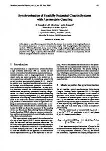
xi (t − 1))| . ∆xi (t) = |x′i (t) − xi (t)| = |F (˜ xi (t − 1)) − F (˜ (11) It has to be stressed that the full nonlinear dynamics contributes to the evolution of ∆xi (t). The spreading of this initially localized disturbance can be characterized in terms of the velocity of information propagation VP [2,4]. As shown in Fig. 2, ∆xi (t) can grow only within a light-cone, determined by Vp . For velocities higher than Vp the disturbance is instead damped. This individuates a sort of predictability “horizon” in space-time: i.e. an interface separating the perturbed from the unperturbed region.

δxi (t + 1) = F ′ (˜ xi (t))[δxi (t) + ε (δxi+1 (t) − 2δxi (t) + δxi−1 (t))] , 2

(13)

where F ′ is the first derivative of a one dimensional chaotic map. Let us again consider as initial condition for the evolution of (13) a localized perturbation as (10) with d0 infinitesimal. The spatio-temporal dynamics of the tangent vector {δxi (t)} is determined by the interaction and competition of two different mechanisms present in Eq. (13): the chaotic instability and the spatial diffusion. As a first approximation, the effects of the two mechanisms can be treated as independent. The chaotic instability leads to an average exponential growth of the infinitesimal disturbance: |δx0 (t)| ≈ d0 exp[λt]. On the other hand, the spatial diffusion, due to the coupling, approximately leads to a spatial Gaussian spreading of the √ disturbance : |δxi (t)| ≈ |δx0 (t)|/ 4πDt exp(−i2 /4Dt) where D = ε/2. Combining these two effects one obtains   i2 1 exp λt − . (14) |δxi (t)| ≈ d0 √ 2εt 2πεt

∆xi(t) 1

300 250 200 10-6 150 t 10-9 100 50 -250-200-150-100 -50 0 50 100 0 150200250 i 10-3

Since the chaotic nature of the phenomenon will typically induces fluctuations, Eq. (14) can only describe the average shape of the disturbance. Moreover, Eq. (14) holds only when the perturbation is infinitesimal, since when

FIG. 2. Evolution of ∆xi (t), for a chain of coupled tent map lattices with a coupling ε = 2/3. The initial perturbation is taken as in (10) with d0 = 10−8 .

4

an intially localized (infinitesimal) disturbance (10) in a reference frame moving with velocity v can be expressed as

the disturbance reaches finite values a saturation mechanism (due to the nonlinearities) sets in preventing the divergence of |δxi (t)|. To verify the validity of (14), we studied the evolution of localized perturbations of a homogeneous spatiotemporal chaotic state, in particular coupled logistic and tent maps have been considered in the regime of “fully developed turbulence” [2]. Firstly, the system is randomly initialized and let to relax for a relatively long transient. At this stage two replicas of the same system are generated and to one of the two a localized perturbation (like (10)) is added. The evolution of the difference field (11) is then monitored at successive times. In order to wash out the fluctuations, the shape of the disturbance is obtained averaging over many distinct realizations.

|δxi (t)| ∼ d0 eΛ(v)t ,

(15)

by following the perturbation along the world line i = vt one can easily measures the corresponding comoving Lyapunov exponent Λ(v) (for more details see [6,22]). The information propagation velocity is the maximal velocity for which a disturbance still propagates without being damped. Therefore it can be defined through the following marginal stability criterion [6]: Λ(VL ) ≡ 0 ,

(16)

where the velocity has been now indicated with VL in order to stress that it has been obtained via a linear analysis. For the maps considered in this section the identity Vp = VL is always fulfilled.

1 -2

10

a

-4

b

10

1 0.8

-8

10

Vp



-6

10

-10

10

0.6 0.4 0.2

-12

10

-14

1

-16

0.8

10

0

400

800 i

2

0

200 i

400 Vp

10

(c)

(d)

(a)

(b)

0

2

FIG. 3. Average evolution of perturbations for a CML of logistic maps (f (x) = 4x(1 − x)) for (a) ε = 1/3 and (b) ε = 1/10. h∆xi (t)i is reported as a function of i2 in a lin-log scale at different times (from bottom to top t = 10, 20, 30, 40). Deviations from a straight line correspond to deviation from the Gaussian shape. h∆xi (t)i is obtained as an average over 103 realizations, for each one ∆xi (0) has been chosen as (10) with d0 = 10−7 . For comparison the prediction (14) is also reported (dashed lines).

0.6 0.4 0.2 0 0

0.2

0.4

0.6

0.8

1 0

0.2

ε

0.4

0.6

0.8

1

ε

FIG. 4. Comparison between the directly measured propagation velocities Vp = VL (circles) and the prediction (18) (boxes) for a CML of logistic maps with (a) a = 3.9 and (b) a = 4, and of tent maps with (c) a = 2 (d) a = 1.8. Lattices of 4 · 104 maps has been used.

As shown in [6], in a closed system with symmetric coupling Λ = Λ(v) has typically a concave shape, with the maximum located at v = 0 (in particular λ = Λ(v = 0)). An approximate expression can be obtained for Λ(v), by substituting i = vt in (14) and by comparing it with (15) :

As one can see from Fig. 3 Eq. (14) is fairly well verified for large enough coupling while it fails at small ε [20]. These discrepancies are due to the finite spatial resolution (that in CML’s is always fixed to 1), since for small diffusivity constant the discretization of the Laplacian becomes inappropriate. The expression (14) for disturbance evolution has been already proposed in Ref. [21] for CML’s in two dimensions. Deviations from (14) have been observed also in [21], but attributed to anomalous diffusive behaviors. It has to be remarked that expression (14) is valid only at short times, since asymptotically (t → ∞) the infinitesimal leading edge of the propagating front |δxi (t)| assumes an exponential profile [11]. For what concerns the propagation velocity, an estimation of Vp can be obtained for infinitesimal perturbations by the evaluation of the so-called maximal comoving Lyapunov exponents Λ(v) [6]. The time evolution of

Λ(v) = λ − v 2 /2ε .

(17)

This parabolic expression for Λ(v) suffers of the same limits mentioned for the Gaussian approximation (14) for the disturbance evolution. Anyway, from (17) an analytical prediction can be obtained for VL : √ VA = 2ελ , (18) which, as shown in Fig. 4, is indeed very good apart from some deviations for ε ≈ 0 and ε ≈ 1. In Sect. V we will 5

reported. As shown in [24], when the coupling ε ≤ 1/2 the maximal Lyapunov exponent for such model coincides with that of the single map (namely, λ = ln(β)) and if β > 1 the system is chaotic. Initially the perturbation, that is still infinitesimal, spreads with the linear velocity VL above defined. At later time it begins to propagate faster with a velocity VP > VL . Comparing Fig. 5 with Fig. 2, one can see that the second stage of the propagation sets in when the bulk of the perturbed region reaches sufficiently high values. As a matter of fact the initial stage of propagation disappears if we initialize the two replicas with a disturbance of amplitude O(1). From these facts it is evident that the origin of the information propagation characterized by Vp > VL should be due to the strong nonlinear effects present in this type of CML.

rederive (18) by assuming that the chaotic perturbation behaves as a front connecting a stable and an unstable (metastable) fixed point in a non-chaotic reaction diffusion system. Let us briefly recall that another method (not suffering for boundary problems) to determine the comoving Lyapunov exponent has been introduced in [22]. The method relies on the computation of specific Lyapunov exponents λ(µ) associated to an exponentially decaying perturbation (with spatial decay rate µ). In other words one assumes that the spatio-temporal evolution of an infinitesimal disturbance can be written as |δxi (t)| ∼ d0 eλ(µ)t−µi .

(19)

Since the asymptotic leading edge of the front separating perturbed from unperturbed part of the chain has an exponential shape, the above assumption (19) is appropriate to study its evolution. It is straightforward to show that the comoving Lyapunov exponents are related to the specific ones via a Legendre transform [22], all the data concerning comoving exponents reported in this paper have been obtained with such a method. Moreover, a further results concerns the linear velocity VL , it can be shown [11] that its value corresponds to the minimal propagation velocity V (µ) = λ(µ)/µ associated with perturbations of the form (19), i.e. VL = min µ

λ(µ) λL ≡ µ µL

∆xi(t) 1 10-3 10-6 10-9 -300 -200 -100

(20)

0 i

where µL and λL = λ(µL ) represent the spatial decay rate and the temporal growth rate of the leading edge, respectively. The expression (20) for the linear velocity is identical to the one derived for propagation of fronts connecting a stable to an unstable steady state [23].

100

200

1400 1200 1000 800 t 600 400 200 0 300

FIG. 5. The same of Fig. 2 for a lattice of coupled shift maps with β = 1.03, ε = 1/3.

The behavior at long times can be understood by considering the dependence of λ(δ) on the disturbance amplitude as shown in Fig. 1b: actually the figure refers to the single map with β = 2, but the shape of λ(δ) is qualitatively the same also for the coupled system and for other β-values. Until the perturbation is infinitesimal λ(δ) ≃ λ and the linear analysis applies, when the disturbance becomes bigger than a certain amplitude, δ N L , the growth will be faster, since now λ(δ) > λ. As it can be clearly seen in Fig. 6, the perturbation is well reproduced by the linear approximation (14) until the amplitude of the perturbation reaches a critical value δ N L ∼ O(10−4 ) above which the nonlinear effects set in. At this stage the nonlinear instabilities begin to push the front leading to an increase of its velocity and deforming the profile of the perturbation. This becomes exponential at much shorter times than in the linear situation discussed in previous subsection. Moreover, when the propagation is dominated by nonlinear mechanisms the spatial decay rate µN L of the asymptotic leading edge will be greater of the linear expected value µL : this result can be explained again invoking the analogy with propagation of fronts connecting

B. Non Linear Mechanisms

In this section we investigate the case of coupled maps for which λ(δ) > λ(0) in some interval of δ. As noticed in Sect. II, this behavior can be observed in chaotic (absolutely unstable) maps, as well as in stable and marginally stable maps. Let us first analyze chaotic maps, nonchaotic ones will be discussed in Sect. IV B. For these systems it is possible to have Vp > VL , this means that the disturbance can still propagate also in the velocity range [VL , Vp ], even if the corresponding comoving Lyapunov exponents are negative. Therefore, the linear marginal stability criterion (16) does not hold anymore. We want to stress that the condition (7) is necessary, but not sufficient to ensure that Vp > VL , since all the details of the coupled model play also an important role. In Fig. 5 the spatio-temporal evolution of an initially localized disturbance of a chain of coupled shift maps is 6

exhibits strong fluctuations. These features suggest that in order to generalize the criterion (16) to nonlinear driven information spreading the growth of finite amplitude perturbations in a moving reference frame should be analyzed.

steady states [11]. 1 -2

10

-4

10

IV. FINITE SIZE LYAPUNOV EXPONENT: EXTENDED SYSTEMS

-6

∆xi(t)

10

-8

10

-10

In this section we introduce the Finite Size Comoving Lyapunov Exponent (FSCLE) that is a generalization of the FSLE to a moving reference frame. First of all let us define the FSLE for an extended system: in this case exactly the same definition given in Sect. II applies, apart from some ambiguities in the choice of the norm to employ for measuring the distance δ(t) of the perturbed, x′ (t) = {x′i (t)}, from the unperturbed replica, x(t) = {xi (t)}. A natural choice could be to perturb randomly x(t) and to look for the doubling times associated to the evolution of the distance

10

-12

10

-14

10

-16

10

0

50

100

150

200

i

FIG. 6. Evolution of the perturbation ∆xi (t) for a CML of shift maps with ε = 1/3 and β = 1.04 at four different times, t = 250, 450, 650, 1000. The solid lines are the expected Gaussian shape (14). The decay rate of the asymptotic exponential profile is µNL ∼ 1.47, noticeably greater than the linear value µL = 0.42.

1 ˜ ∆(t) = L

1

i=−L/2

|x′i (t) − xi (t)| ;

(21)

an alternative choice consists in perturbing a single site of the chain, let’s say i = 0, at time t = 0 and to evaluate the “single site” norm

10-2 10-4 10-6 ∆xi(t)

L/2 X

∆x0 (t) = |x′0 (t) − x0 (t)|

10-8

(22)

We have verified that the two norms (21) and (22) give equivalent results for what concerns the evaluation of λ(δ). In this paper we will limit to consider the norm (22). In order to measure the FSCLE in a reference frame moving with velocity v, we have simply measured the difference (22) along a world line i = vt; i.e.

10-10 -12

10

10-14 10-16 10-18 0

.

200 400 600 800 1000 1200 1400 1600 1800 2000 t

∆xic +[vt] (t) = |x′ic +[vt] (t) − xic +[vt] (t)| .

FIG. 7. Time evolution of ∆x0 (t) (solid line) and ∆xi (t) (dashed line), for i = V2 t with V2 = 1/3. In this last case the data for two different chain configurations are reported. The map used is the shift map with β = 1.1, ε = 1/3 and L = 2 · 103 . For these parameters one has VL = 0.250 and Vp = 0.342. Note that between t = 200 and t = 500 for ∆xi (t) the numerical precision is reached.

(23)

where [ · ] denotes the integer part and ic is introduced below. The FSCLE is then estimated as in Sect. II. Once a set of thresholds δn = rn δ0 , with n = 0, . . . , N , is chosen and the perturbation is initialized as ∆xi (0) = δmin δi,0 with δmin ≪ δ0 . A preliminary transient evolution is performed in order to allow to the perturbed orbit to relax on the attractor. At the end of this short transient the position ic where the perturbation reaches its maximum is detected, this point is taken as the vertex of the light cone from which all the considered world lines i = v t depart. The FSCLE is then defined as    1 ∆ Λ(δn , v) = log , (24) hτ (δn )ie δn e

To better clarify the difference between the linear and non linear mechanisms we show the behavior of ∆xi (t) along the world line i = V t for two different velocities: V1 = 0 and VL < V2 < Vp . From Fig. 7, one observes for the zero-velocity situation an exponential increase of the perturbation with rate λ until it eventually saturates. For the case corresponding to velocity V2 an initial exponential decay with rate Λ(V2 ) is seen, followed at later times by a resurgence of the disturbance. The successive evolution of the perturbation is no more exponential and 7

In the interval VL ≤ v ≤ Vp (see Fig. 8(b)), Λ(δ, v) is still positive and its maximal value decreases for increasing v. The FSCLE vanishes for v = Vp as Fig. 9 (a) shows. In this velocity range Λ(v) is always negative, therefore the instabilities observed in a reference frame moving with velocity higher than VL have a fully nonlinear origin. The residual fluctuations present in Λ(δ, v) are essentially due to the limited statistics. Indeed the nonlinear growth as shown in Fig. 7 is extremely fluctuating.

where the dependence on the velocity v derives from the employed norm (23). Note that we have used Eq. (4) due to the discreteness of the temporal evolution. In the limit of very small perturbation the FSCLE reduces to the comoving Lyapunov exponent lim Λ(δ, v) = Λ(v) ,

δ→0

(25)

and, for v = 0 one has the FSLE λ(δ). Actually there are finite time effects which prevents the limit (25) to be correctly attained. This is related to the fact that the FSCLE’s can be obtained only via finite time measurements. In the Appendix we show how one can include such finite time corrections. In the next subsections we will give evidences that the marginal linear stability criterion (16) can be generalized with the aid of the FSCLE in the following way: δ

for v ≥ Vp ,

0.45

a

0.4 0.35 0.3 Λ(δ,v)

max{Λ(δ, v)} = 0

0.5

(26)

0.25 0.2 0.15

where Vp can be either VL , if the information propagation is due to linear mechanisms, or greater than VL , when nonlinear mechanisms prevail on the linear ones. For v > Vp one has Λ(δ, v) = 0, since due to the definition of the FSCLE negative growth rate appear to be 0.

0.1 0.05 0 10-7

10-6

10-5

10-4

10-3

10-2

10-1

1

δ 0.25

A. Chaotic Systems

b

0.2

Let us first consider chaotic systems for which Vp ≡ VL , in this case

Λ(δ,v)

0.15

max{Λ(δ, v)} = Λ(v)

0.1

δ

and the generalized criterion (26) reduces to the linear one (16). As already stressed in Sect. III B, shift coupled maps represent a prototype of the class of chaotic models for which Vp can be eventually bigger than VL . For this model the behavior of Λ(δ, v) for various velocities is reported in Fig. 8. For v < VL , we observe that Λ(δ, v) ∼ Λ(v) up to a certain value of the disturbance amplitude δ N L , above which the FSCLE increases and exhibits a clear peak at some higher δ-value. From Fig. 8 (a) it is clear that δ N L (which denotes the set in of the regime dominated by nonlinear mechanisms) decreases for increasing velocities and finally vanishes at v = VL . This behavior is reasonable since, as shown in Fig. 5, initially the disturbance evolves along the chain following the linear mechanism characterized by Λ(v), but as soon as in the central site δ > δ N L the nonlinear mechanism begins to be active. Thus a nonlinear front is excited and this invades the linear region propagating with a velocity higher than VL , therefore the higher is v the smaller is the scale at which nonlinear effects are observed.

0.05

0 10-7

10-6

10-5

10-4

10-3

10-2

10-1

1

δ

FIG. 8. Λ(δ, v) as a function δ for various velocities. The data refer to the coupled shift maps with β = 1.1 and ε = 1/3, with these parameters VL ∼ 0.250 and Vp ∼ 0.342. In (a) results for velocities v < VL are reported, namely (from top to bottom) v = 0, v = 0.10 and v = 0.16. The straight lines indicate Λ(v). In (b) velocities in the range [VL : Vp ] are reported, from the top v = 0.25, v = 0.286, v = 0.30, v = 0.33, v = 0.34. Chains of lengths from L = 104 up to L = 105 have been employed and the statistics is over 2 · 103 doubling times.

In Figure 9(a) the dependence of maxδ {Λ(δ, v)} on v for coupled shift maps is reported, as expected it vanishes exactly for v = Vp . For v < VL a non-monotonous behavior of maxδ {Λ(δ, v)} is observable, this is probably due to the complex interplay of linear and nonlinear effects. For v > VL , the behavior is smoother and a monotonous 8

limit v → Vp Λ(δ, v) → 0, as shown in Fig. 9 (b). At variance with the shift map (that is an everywhere expanding map) the considered map shows contracting and expanding intervals. Therefore the disturbances during their spatio-temporal evolution can be alternatively expanded or contracted. This leads to strong fluctuations in the FSCLE-values, that are difficult to remove. As a matter of fact we observed that even for velocities slightly larger than Vp Λ(δ, v) can be non zero. But the statistics of these anomalous fluctuations is extremely low, referring to the parameters reported in Fig. 9 (b) for v = 0.6 > Vp = 0.59 we observed an expansion (instead of the expected contraction) of disturbances in the 0.5% of the studied cases. For higher velocities Λ(δ, v) is zero for any considered δ.

decrease is observed. As discussed in Sect. II, the discontinuity present in the shift map is not necessary in order to observe nonlinear mechanisms prevailing on linear ones. As an example of continuous map exhibiting an information propagation velocity Vp > VL the map (8) is considered. This type of CML has been already studied in [10]: it has been observed that in a certain parameter range Vp can be finite even if the map is non chaotic. Moreover, also in the chaotic regime there is a window of parameters where Vp > VL , with our parameters choice λ ≈ 0.182 > 0. 0.5 0.4

a maxδ[Λ(δ,v)]

0.3

B. Non Chaotic Systems

0.2

On the basis of the linear analysis discussed in Sect. III A the propagation of disturbances should be present only in chaotic systems. For non chaotic ones λ ≤ 0 and from Eq. (16) one trivially obtains VL = 0. On the other hand, in the class of systems for which λ(δ) ≥ λ there are also stable and marginally stable systems. Therefore, a propagation due solely to non linear terms can still be present [9–11]. In this section we want to discuss the possible employ of the FSLE to characterize these maps. Before entering into the description of the FSLE computation in such systems, it is of interest to recall an important phenomenon which appears in stable systems: the so-called “stable chaos” [9]. Stable systems asymptotically evolve towards trivial attractors (i.e. fixed points, periodic or quasi-periodic orbits). However, in spatially extended systems it may happen that the time needed to reach the asymptotic state is very long: it has been found that in certain stable CML the transient time diverges exponentially with the number of elements of the chain [8]. Moreover, this transient is characterized by a quasi-stationary behavior allowing for the investigation of the properties of the model with statistical consistency. In Ref. [9] it has been shown that a chain of coupled maps of the type (8), considered in their discontinuous limit (i.e. for c → ∞), is non chaotic but still exhibits erratic behaviors. This is associated to a non-zero information spreading within the system. As far as the computation of the FSLE for these systems is concerned, some remarks are worth to be done. The definition of the FSLE in term of error doubling times cannot be used in a straightforward manner to determine negative expansion rates. Another important point is that, at variance with the case of chaotic maps, finite perturbations should be now considered in order to observe an expansion. These two points impede a straightforward implementation of our method to study these systems. Indeed, if

0.1 0 -0.1

VL

Vp

-0.2 0

0.05

0.1

0.15

0.2

0.25

0.3

0.35

v 0.7 0.6

b

maxδ[Λ(δ,v)]

0.5 0.4 0.3 0.2 0.1 0

VL

-0.1

Vp

-0.2 0

0.1

0.2

0.3

0.4

0.5

0.6

v

FIG. 9. maxδ Λ(δ, v) (dashed line with points) versus v compared with Λ(v) (continuous line). (a) Results for coupled shift maps with the same parameters as Fig. 8, the vertical lines indicates VL ≈ 0.250 and the measured (12) propagation velocity Vp ≈ 0.342. (b) Data for the coupled maps (8) with parameters b = 2.7, d = 0.1, q = 0.07 and c = 500 and with coupling ε = 2/3, the vertical lines indicates VL ≈ 0.39 and Vp ≈ 0.59. In this second case chains of length L = 2 · 104 have been considered and the statistics is over 2 · 104 doubling times. The reported values for maxδ Λ(δ, v) refer to an average over five values of δ around the peak position of Λ(δ, v).

Also in the present case we observe an overall behavior of the FSCLE resembling that of the coupled shift maps. The main point that we want to remark is that in the 9

result is in good agreement with the one obtained in [19] and confirms that at the origin of the perturbation propagation in this system there should be a mechanism very similar to the one discussed for the shift map. Further studies related to the “stable chaos” phenomenon have been recently performed [26].

one starts with too small perturbations the propagation does not manifest, while if one initializes the system with a finite perturbation λ(δ) cannot be estimated with the required accuracy. Indeed, the only way to have an independence of λ(δ) from the initial conditions is to initialize the system with infinitesimal perturbations and then to follow them until they become finite due to the dynamics of the system (see Ref. [14] for a detailed discussion). The coupled (8) maps for c → ∞ have been recently analyzed by Letz & Kantz [19] in term of an indicator similar to the FSLE (i.e. able to quantify the growth rate of non infinitesimal perturbations). This indicator turns out to be negative for infinitesimal perturbations and becomes positive for finite perturbations. This means that a finite perturbation of sufficient amplitude can propagate along the system due to nonlinear effects. This confirms what was previously observed in Ref. [11] for marginally stable systems.

V. ANALOGIES WITH FRONT PROPAGATION IN REACTION DIFFUSIONS SYSTEMS

The perturbation evolution in spatially distributed systems can be described as the motion of an interface separating perturbed from unperturbed regions. In this spirit, one can wonder if and to what extent it is possible to draw an analogy between the evolution of this kind of interface and the propagation of fronts connecting steady states in reaction diffusion systems. As already noticed in Ref. [11], the two phenomena display many similarities. In the following we will discuss the similarities and differences, in particular we will introduce a simple phenomenological model which can help us in highlighting the analogies. Let us start by recalling the basic features of fronts propagation in reaction diffusion systems with reference to the Fisher-Kolmogorov-Petrovsky-Piscounov (FKPP) equation [16]

1

Ι(δ)

0.6

f(x)

0.8

0.4

1 0.8 0.6 0.4 0.2 0 0 0.20.40.60.8 1 x

0.2

2 ∂t θ(z, t) = D∂zz θ(z, t) + G(θ(z, t)) ,

(27)

0 -0.2 10-7

10-6

10-5

10-4

10-3

10-2

10-1

where θ(z, t) represents the concentration of a reactants which diffuses and reacts, the chemical kinetics is given by G(θ). Typically the function G(θ) ∈ C 1 [0, 1] (with G(0) = G(1) = 0) exhibits one stable (θ = 1) and one unstable (θ = 0) fixed point. Once the system is prepared on the stable state (θ(z) = 0 ∀z), an initial (sufficiently steep) perturbation (e.g. a step function θ(z, t = 0) = Θ(z − z0 ) ) will give rise to a smooth front moving with a velocity Vp , that will connect the unstable and the stable fixed points: as a result the stable state will invade the unstable one. This equation admits many different traveling solutions that are typically characterized by their propagation velocities, however for a sufficiently steep initial perturbation of the unstable state the selected front is unique and its velocity Vp is bounded in the interval [Vmin , Vmax ], where q Vmin = 2 DG′ (0) (28)

100

δ

FIG. 10. I(δ) as a function of the amplitude perturbation in a lin-log scale for the discontinuous coupled maps (8), in the limit c → ∞, with ε = 1/3 and L = 35. The map is reported in the inset. The negative maximal Lyapunov λ = −0.105 is recovered at small scales. For the computation details see the text. In the inset the single map is shown.

In Fig. 10 we show the behavior of a quantity I(δn ) similar to λ(δn ) which has been obtained as follows. We considered two trajectories at an initial distance δn , after one time step evolution the distance δ between the trajectory is measured. Then one of the two trajectory is rescaled at a distance δn from the other, keeping the direction of the perturbation unchanged, and the procedure is repeated several times and for several values of δn . Then we averaged ln(δ/δn ) over many different initial conditions obtaining I(δn ). For δn → 0, this is nothing but the usual algorithm for computing the maximal Lyapunov exponent [25]. As discussed in Ref. [14] this method suffers of the problem that when δn is finite one is not sure to sample correctly the measure on the statistically stationary state. Indeed a finite perturbation will generically bring the trajectory out from the “attractor”. Nevertheless the

and

s

Vmax = 2 D sup

0 A an increase of Vp with respect to Va is observed.

0.8 0.7 0.6 0.5 V

0.45 0.4 0.3

0.4

0.2 0.35 Vp

0.1 0

0.3

1

1.1

1.2

1.3

1.4

1.5

1.6

1.7

1.8

1.9

β

FIG. 13. Information propagation velocities for the shift map with ε = 1/3: (boxes) linear velocities VL and (crosses) directly measured nonlinear ones. The two lines correspond to Va (18) (dotted line) and to the propagation velocity for the model (30) with λ(u) given p by (6) (solid line). The dashed curve with asterisks is Vs = 2ε maxδ {λ(δ)}.

0.25

0.2 10-6

10-5

10-4

10-3

10-2

10-1

1

NL

δ

FIG. 12. Propagation velocities Vp as a function of δ NL for the model (30), (34) with ε = 1/3, A = ln(1.1), B = ln(1.3), C = A, δ0sat = 0.53. The crosses refer to the case δ sat = δ0sat , sat NL while the boxes to the = δ0sat √ case δ √ + δ . The two lines correspond to Va = 2εA and Vs = 2εB.

The FSLE for coupled shift maps is actually different from (6), but we are neglecting correlations among different sites and effects due to the specific measure associated to the system. Nevertheless, a numerical integration of Eq. (30) equipped with (6) reproduces semiquantitatively the features observed for a lattice of coupled shift maps (see Fig. 13). In particular, also the simple mean-field model (30) with the choice (6) is able to forecast the observed transition from nonlinear to linear behavior for β → 2.

In the whole examined parameter range Vp is always reasonably approximated by Vs , but smaller. By increasing B one observes an increase of the difference between the measured velocity and the linear prediction. These results confirm that the condition (7) is indeed a necessary condition in order to observe nonlinear propagation of information. We will now investigate the role of δ N L in determining the propagation velocity. It is quite obvious that modeling the dynamics via the Eqs. (30) and (34) the nonlinear effects will disappear in the limit δN L → δ sat and this is indeed confirmed by the simulations (see Fig. 12). In order to examine a less obvious situation, a modification of the expression (34) is also considered. In this second case δ sat = δ0sat + δ N L is assumed, therefore by varying δ N L the extension of the amplitude interval over which the

Concluding this section we can safely affirm that (30) is a reasonable model to mimic the perturbation evolution at a mean field level, neglecting the spatio-temporal fluctuations and correlations. In the same fashion λ(u) can be considered as an “effective” non linear kinetics for the perturbation evolution.

12

ACKNOWLEDGMENTS

VI. FINAL REMARKS

Stimulating interactions with F. Cecconi, R. Livi, K. Kaneko, A. Pikovsky, A. Politi, and A. Vulpiani are gratefully acknowledged. Part of this work has been developed at the Institute of Scientific Interchange in Torino, during the workshop on “Complexity and Chaos” in October 1999. We acknowledge CINECA in Bologna and INFM for providing us access to the parallel CRAY T3E computer under the grant “Iniziativa Calcolo Parallelo”.

In this paper information (error) propagation in extended chaotic systems has been studied in details. In particular, we have analyzed the relevance of linear and nonlinear mechanisms for the propagation phenomena in spatio-temporal chaotic coupled map lattices. Linear stability analysis is not always able to fully characterize disturbance propagation. This is particularly true for (marginally) stable systems with strong nonlinearities, where finite size perturbations are responsible for information spreading in the system. When the nonlinear effects prevail on the linear ones the propagation velocity of information Vp can be higher than the linear velocity VL . A necessary condition for the occurrence of information spreading induced by nonlinear mechanisms has been expressed in terms of the Finite Size Lyapunov Exponent (FSLE). We have also shown the existence of strong analogies between error propagation and front propagation in reaction-diffusion models. In particular, the above mentioned necessary condition is analogous to the Aronson & Weinberger theorem [27] for front connecting stable and unstable steady states. In the linear and nonlinear case, the propagation velocity Vp can be identified via an unique marginal stability criterion involving Finite Size Lyapunov Exponents defined in a moving reference frame. This result generalizes the corresponding linear criterion expressed in terms of the maximal comoving Lyapunov exponents for the identification of VL [6].

APPENDIX A:

In any numerical computation of the Lyapunov exponents one is forced to use a finite time approximation for an infinite time limit. Nevertheless, provided that the convergence to the asymptotic value is fast enough, this is not a dramatic problem. As a matter of fact, in low dimensional systems very fast convergence to the asymptotic value is usually observed. However, this problem manifest more dramatically in high dimensional systems, where the time to align along the direction of maximal expansion could be very long [29,33,34]. In the present case this problem is complicated by the fact that the FSLE is intrinsically a finite time indicator. Indeed the time a perturbation takes to grow from a value δ to rδ is finite unless δ → 0. However, for the CML models here analyzed and for initially localized perturbation (10) it is possible to evaluate the corrections to apply to the FSCLE, estimated at finite time, in order to recover, for sufficiently small δ, the expected limit Λ(v). These corrections allow for a faster convergence of the FSCLE to its asymptotic values. For the sake of simplicity we consider maps with constant slope, e.g. the shift map F (x) = β x mod 1, and the CML defined in Eq. (9). In this case (for ε < 1/2) the maximal Lyapunov exponent of the CML coincides with that of the single map [24]; i.e. λ = ln β. We will limit to the case v = 0 (i.e to the FSLE), since the extension to generic v is straightforward. As shown in [33,35] the finite time evolution of an infinitesimal perturbation d0 initially localized in i = 0 can be expressed at time T as the sum of the contributions M (m, T ) associated to all the paths connecting the space-time point (i = 0, t = 0) to the point (i = 0, t = T ), i.e.

These results can be of some interest for the synchronization and the control of extended systems. It has been recently shown that the synchronization of coupled extended systems is strongly influenced by nonlinear effects. In particular, the synchronization time exponentially diverges with the system size, even in non-chaotic situations, provided that Vp > 0 [30]. We believe that in these systems the appropriate indicator to characterize such transition would be the “transverse” Lyapunov exponent [31], once extended to finite scales. As far as control schemes are concerned, since they rely mainly on linear analysis [32], new nonlinear methods (e.g. based on the concept of FSLEs) should be introduced in order to control the erratic behaviors due to fully nonlinear mechanisms.

T X δxi=0 (T ) = βT M (m, T ) . d0 m=0

A further aspect that should be addressed in future work concerns the extension of the applicability of the FSLE also to linearly stable systems: a candidate in this respect could be the indicator recently introduced in [19].

(A1)

where m is the number of “diagonal links” connecting (i, t) to (i ± 1, t + 1) present in the path of length T . Each path [m, T ] of length T with m diagonal links contributes to the above sum with a term  ε m (1 − ε)T −m (A2) M (m, T ) = N (m, T ) 2

Finally, it is reasonable to expect that the present analysis is not limited to discrete models but that it can be applied to continuous extended systems described in terms of PDE’s, e.g. to the complex Ginzburg-Landau equation. 13

where N (m, T ) is the multiplicity associated to each path [m, T ] (for more details see [35]). As can see from Eq. (A1) the finite time Lyapunov exponent λT will be given by T 1 X 1 δx0 (T ) = ln β + ln M (m, T ) . λT = ln T d0 T

[8] J.P. Crutchfield and K. Kaneko, Phys. Rev. Lett. 60, 2715 (1988). [9] A. Politi, R. Livi, G.L. Oppo and R. Kapral, Europhys. Lett. 22, 571 (1993). [10] A. Politi and A. Torcini, Europhys. Lett. 28, 545 (1994). [11] A. Torcini, P. Grassberger and A. Politi, J. Phys. A27, 4533 (1995). [12] M. Cencini, M. Falcioni, D. Vergni and A. Vulpiani, Physica D 130, 58 (1999). [13] U. Dressler and J.D. Farmer, Physica D 59, 365 (1992); T.J. Taylor, Nonlinearity 6, 369 (1993). [14] E. Aurell, G. Boffetta, A. Crisanti, G. Paladin and A. Vulpiani, Phys. Rev. Lett. 77, 1262 (1996); J. Phys. A30, 1 (1997). [15] I. Waller and R. Kapral, Phys. Rev. A 30 , 2047 (1984); K. Kaneko, Prog. Theor. Phys. 72, 980 (1984). [16] R.A. Fisher, Ann. Eugenics 7, 355 (1937); A.N. Kolmogorov, I. Petrovsky and N. Piscounov, Bull. Univ. Moscow, Ser. Int. A1, 1 (1937). [17] U. Ebert and W. van Saarloos, Physica D 146, 1 (2000). [18] A recent review on the subject is G. Boffetta, M. Cencini, M. Falcioni and A. Vulpiani, unpublished (nlin.CD/0101029). [19] T. Letz and H. Kantz, Phys. Rev. E 61, 2533 (2000). [20] Note that also for ε → 1 deviations are observed. This is due to the fact that for ε = 1 the system reduces to two uncoupled subchains, therefore also for ε ∼ 1 the coupling among nearest neighbors is actually very small. [21] W. van de Water and T. Bohr, Chaos 3, 747 (1993). [22] A. Politi and A. Torcini, Chaos 2, 293 (1992). [23] W. van Saarloos, Phys. Rev. A 37, 211 (1988); ibidem, 39, 6367 (1989). [24] S. Isola, A. Politi, S. Ruffo, and A. Torcini, Phys. Lett. A, 143, 365 (1990). [25] I. Shimada and T. Nagashima, Prog. Theor. Phys. 61, 1605 (1979); G. Benettin, L. Galgani, A. Giorgilli and J.M. Strelcyn, Meccanica, March 15 and 21 (1980). [26] F. Ginelli, R. Livi, and A. Politi, private communication. [27] D.G. Aronson and H.F. Weinberger, Adv. Phys. 30, 33 (1978). [28] J. Armero, J. Casademunt, L. Ram´irez-Piscina, and J.M. Sancho, Phys. Rev. E 58, 5494 (1998); A. Rocco, U. Ebert, and W. van Saarloos, Phys. Rev. E 62, R13 (2000). [29] A.S. Pikovsky and J. Kurths, Phys. Rev. E 49, 898 (1994). [30] L. Baroni, R. Livi, and A. Torcini, accepted for publication on Phys. Rev. E , it will appear in the volume of March 2001 (nlin.CD/0003010). [31] L.M. Pecora and T.L. Carroll, Phys. Rev. Lett. 64 821 (1990). [32] E. Ott, C. Grebogi, and J.A. Yorke, Phys. Rev. Lett. 64, 1196 (1990). [33] A. Pikovsky, Chaos 3, 225 (1993). [34] I. Goldhirsh, P.L. Sulem and S.A. Orszag, Physica D 27, 311 (1987). [35] R. Livi, S. Ruffo, and A. Politi, J. Phys. A 25, 4813 (1992); A. Torcini, R. Livi, S. Ruffo, and A. Politi, Phys. Rev. Lett. 78, 1391 (1997).

m=0

(A3)

the first contribution is the asymptotic one, while the second one will vanish in the limit T → ∞ and it is the finite-time correction to evaluate. This second contribution can be numerically estimated by considering the finite time evolution of the Lyapunov eigenvector {Wi (t)} associated to the maximal Lyapunov exponent, once it is initialized as Wi (0) = d0 δi,0 . The evolution of {Wi (t)} in the tangent space is ruled by the following equation i h ε Wi (t + 1) = β (1 − ε)Wi (t) + (Wi−1 (t) + Wi+1 (t)) . 2 (A4) In order to evaluate the finite time corrections, one should iterate at the same time Eq. (A4) (with β fixed to one) and the two replicas required for computing λ(δ) (see Sect. II). Then the estimation of the FSLE should modified in the following way:    1 |δxi (t + τ (δn , r))| λ(δ) = ln hτ (δn , r)ie |δxi (t)|   |Wi (t + τ (δn , r))| . (A5) − ln |Wi (t)| e The case of maps with non constant slope is computationally much heavier. Since for each different path the local ′ multiplier F (x˜i ) will be different and they will depend on the particular trajectory under consideration [33,35]. As a matter of fact we have observed that if the multipliers are equally distributed among positive and negative values, the finite time corrections essentially cancel out.

[1] [2] [3] [4] [5] [6]

R. Shaw, Z. Naturf. 36a, 80 (1981). K. Kaneko, Physica D 23, 436 (1986). T. Bohr and D. Rand, Physica D 52, 532 (1987). P. Grassberger, Physica Scripta 40, 346 (1989). G. Paladin and A. Vulpiani, J. Phys. A27, 4911 (1994). R.J. Deissler and K. Kaneko, Phys. Lett. A119, 397 (1987). [7] S. Lepri, A. Politi and A. Torcini, J. Stat. Phys., 82 (1996) 1429; J. Stat. Phys., 88 (1997) 31; Chaos, 7 (1997) 701.

14