Linear Boundary Extensions for Finite Length Signals ... - IEEE Xplore

IEEE TRANSACTIONS ON SIGNAL PROCESSING, VOL. 52, NO. 11, NOVEMBER 2004

3213

Linear Boundary Extensions for Finite Length Signals and Paraunitary Two-Channel Filterbanks María Elena Domínguez Jiménez and Nuria González Prelcic, Member, IEEE

Abstract—In this paper, we introduce a novel and general matrix formulation of artificial linear boundary extension methods for removing border effects inherent to any paraunitary two-channel size-limited filterbank. This new characterization of the transformation operator allows us to prove that perfect reconstruction (PR) of finite signals can be ensured under some conditions without using extra subband coefficients; in other words, we characterize the signal extension methods that lead to nonexpansive transforms. The necessary and sufficient condition we find allows us to show that some traditional extension techniques that are being used in an expansive way, such as the polynomial extension, lead in fact to nonexpansive invertible transforms; moreover, we can also prove that in contradiction to previous literature, not every transformation matrix associated with a linear extension is invertible even if using prototype filters of the same length. Apart from these invertibility criteria, we propose the first algorithm for the design of all linear extensions and their associated biorthogonal boundary filters that lead to nonexpansive and invertible transforms. Analogously, we provide the first method for the design of all linear extensions that yield orthogonal transforms: We construct an infinite number of orthogonal extensions, apart from the commonly used periodic extension, and their associated orthogonal boundary filters. The final contribution of the paper is a new algorithm for the design of smooth orthogonal extensions, which keep the orthogonality property and overcome the main drawback of periodization, that is, the introduction of subband coefficients of great amplitude near the boundaries in the transform domain. Index Terms—Border effects, boundary extensions, orthogonal transforms, smooth orthogonal extensions, two-channel filterbanks.

I. INTRODUCTION

T

WO channel finite impulse response (FIR) filterbanks have been extensively studied in the literature [1]–[5] since they constitute the basic cell of tree-structured filterbanks. Their design and relationship to wavelet and wavelet packet transforms [6]–[13] are well understood when processing signals of infinite extension. However, in a wide range of areas, it is necessary to handle discrete finite length signals such as audio and speech signals, electrocardiograms (ECGs), images, time series (in economy, meteorology, seismography, etc), as well as the discretizations

Manuscript received November 25, 2002; revised October 2, 2003. This work was supported by CICYT under Project TIC200-3697-C03-01. The associate editor coordinating the review of this paper and approving it for publication was Prof. Trac. D. Tran. M. E. Domínguez Jiménez is with Departamento de Matemática Aplicada a la Ingeniería Industrial, Universidad Politecnica de Madrid, Madrid, Spain (e-mail: [email protected]). N. González Prelcic is with the Departamento de Teoría de la Señal y las Comunicaciones, Universidad de Vigo, Vigo, Spain (e-mail: [email protected]). Digital Object Identifier 10.1109/TSP.2004.836526

of continuous functions of compact support (for instance, the solutions of discretized differential equations with boundary conditions). Hence, applications of subband processing of finite signals include, but are not limited to, image compression, audio coding, subband adaptive equalization, multicarrier modulation systems, CDMA schemes, and ordinary and partial differential equations [14]–[24]. Filterbank theory and wavelet transforms thus had to be modified to be applied to finite sequences or compact support functions, respectively. To clearly understand this problem, first of all, we need to consider the operation of the two channel filterbank on an infinite signal column vector ; this can be formulated by using the infinite transformation matrix defined in (1), shown at the bottom of the next page, and are the length- lowpass and highpass where analysis filters, respectively. When this kind of operator has to be applied to finite signals, the first idea one thinks of , but it is well known that if is to truncate the matrix no extra processing is applied, border distortions will appear in the reconstructed signal [11], [25], [26]. To remove this artifact, two different approaches have been pointed out: a) artificial extension at the boundaries of the finite signal before the analysis stage [26]–[29] and b) design of border filters or wavelets on the interval [30]–[32]. As we will see later on, both approaches may be merged into one since the first type of method also leads to the construction of specific border filters. Despite recent advancements along these lines [21], [27]–[29], [31]–[33], filterbank theory for finite length signals is still an open subject. In the papers included in the first approach, we have observed some unsolved matters. • In several practical applications, only the traditional extension methods are used: periodization, symmetric extension, and zero padding [11]. For instance, in image coding, the JPEG2000 Standard [21] applies symmetric extension at the boundaries of the image because it processes each row or column vector via linear-phase filters [27]. However, for other applications where orthogonality is desired (for example, audio coding, subband adaptive equalization, CDMA schemes, and some differential equations with boundary conditions), it is necessary to use tree-structured paraunitary filterbanks (which have no linear phase), and symmetric extension may not fulfill the perfect reconstruction (PR) property. This is the reason why in this paper, we will focus on paraunitary two-channel filterbanks and will define alternative boundary extension methods for such applications. As an example of this, we will propose polynomial extension,

1053-587X/04$20.00 © 2004 IEEE

3214

IEEE TRANSACTIONS ON SIGNAL PROCESSING, VOL. 52, NO. 11, NOVEMBER 2004

•

•

•

•

which is a generalization of the so-called linear and quadratic extrapolation [11]. A simple theoretical matrix formulation that is common to all signal extension methods, including the classical extension techniques, is lacking. Some works [26], [28] provide expressions for the subband transforms associated to signal extensions, but they are not the most generalized ones, since they only consider that, at each border, the artificially appended samples solely depend on the original samples at the same border. Therefore, signal extensions similar to periodic extension are not included in their formulation. In [34], a general expression is given, but the matrix operator is not explicitly obtained. Thus, in Section II, we will show the most generalized expression of the transform matrix, the entries of which appear by means and and the extension of the prototype filters matrices. Except for symmetric extension (when using linear phase filters) and periodic extension, the rest of the extensions (zero padding, polynomial extension) are used in an expansive way, that is, to achieve PR, more transform domain coefficients are needed than samples in the original signal. Considering paraunitary filterbanks, it seems that periodization is the unique nonexpansive extension technique, that is, the only one which assures PR. However, in Section III, we will characterize all nonexpansive extension methods and demonstrate that polynomial extension is also nonexpansive. Given a filterbank, the issue concerning the existence or nonexistence of extension methods for which the associated transform is not invertible is still open. In effect, invertibility assumptions need to be imposed [26], [28], [34], [35] in order to assure PR at the synthesis stage. In [33], one can find an example of a signal extension that yields a non invertible transform; therefore, PR is not always achieved. However, in the same paper, it is stated that the method has been shown empirically to be consistent for all uniform-length filterbanks tested, and it is suggested that it may always work for -channel filterbanks whose filters have the same length. In contradiction to this conjecture, in Section III, we construct, for any two-channel paraunitary filterbank constituted by filters of the same even length, an infinite number of signal extension techniques for which the transformation matrices are not invertible. Absence of an algorithm for the design of linear nonexpansive invertible transforms: In the previous literature, there are neither results that specifically deal with how many in-

.. .

.. .

vertible transforms associated with signal extensions can be built nor how to design them. Therefore, as one of the main contributions of this paper, in Section IV, we provide the first method for designing all nonexpansive signal extension techniques. • Nonexistence of orthogonal extensions apart from the periodic extension: As already mentioned, in the applications where orthogonality is desired (audio coding, CDMA, differential equations), only paraunitary filterbanks can be used. In these cases, periodic extension is apparently the only extension technique that leads to an orthogonal transform. Nevertheless, in Section V, we will show that there are infinitely many orthogonal transforms, and the first algorithm for their design will be introduced. This constitutes one of the main purposes of our work. • Many of the commonly used extension techniques introduce artificial high frequencies at the borders of the transform vector, as described in [25]. Symmetric extension does not produce discontinuities in the extended signal, but it introduces jumps in its first derivative, which provoke artificial highpass coefficients of great amplitude. This is a very annoying effect in some applications, such as audio coding. To avoid these effects, we propose polynomial extension as an alternative smooth technique; besides, it achieves PR when using paraunitary filterbanks, as it is proven in Section III-B1. • To summarize, the most important motivation for our work lies in the fact that smooth orthogonal extensions have never been obtained before. The interest of such techniques is without a doubt in their applications to audio coding and subband equalization, where orthogonality is desired, and spurious high frequencies must be avoided. So far, periodization was the unique orthogonal extension technique, but it is not smooth, since the periodization process creates artificial discontinuities. Thanks to our formulation, in Section V-A, we present our final result: a novel method for the design of smooth orthogonal extensions that is adaptive to each finite signal. Concerning the second approach, the basic research on the design of border filters for finite signals is due to Herley and Vetterli [31]. In their paper, a set of boundary orthogonal filters is constructed by means of the orthogonalization process of a . They show that the finite matrix with the same structure as first and the last rows of the resulting matrix (being the length of the prototype filters) correspond, respectively, to the left and right boundary filters, but this algorithm only generates a particular case of border filters: the ones that present, coefficients. Besides, the design algorithm does at most,

.. .

.. .

.. .

.. .

.. . (1)

.. .

.. .

.. .

.. .

.. .

.. .

.. .

DOMÍNGUEZ JIMÉNEZ AND GONZÁLEZ PRELCIC: LINEAR BOUNDARY EXTENSIONS FOR FINITE LENGTH SIGNALS

not have any mechanism to control the possible introduction, in the transform domain, of the previously mentioned artificial high frequencies. However, in Section VI, we will explain how our formulation provides all sets of orthogonal and biorthogonal boundary filters. On the other hand, the methods we propose are not iterative, since the boundary filters are given in a closed form. Moreover, for the orthogonal case, the numerical errors remain bounded, and the computational cost is small. The recent advances in design techniques of boundary filters provide alternative orthogonal solutions [36], but the problem of the appearance of spurious high frequencies seems to remain unsolved. To this aim, in Section V-B, we will finally apply our theoretical results about orthogonal smooth extensions. Some illustrative examples will show that the new proposed technique yields even better results than the optimized orthogonal boundary filters obtained in [36]. In summary, this paper is focused on artificial extension methods for processing finite-length signals via paraunitary two-channel filterbanks, introducing a novel theoretical formulation that helps us to solve some of the existing problems and lacks. It is organized as follows: Section II starts with the presentation of some preliminary observations that are necessary to follow the development of the matrix operator, which constitutes the fundamental mathematical tool for the rest of the paper. Section III shows how the new matrix formulation allows us to obtain the conditions to be satisfied by the extension technique to ensure perfect reconstruction of finite signals without resorting to extra subband samples; counterexamples to the results presented in previous works, which ensure that the transformation matrix is always invertible whenever it is associated with prototype filters of equal length, are also included; next, we prove that techniques that have been previously classified as expansive lead, in fact, to nonexpansive transforms; moreover, for such invertible classical extensions, we show that the borders of the original signal can be uniquely recovered from the borders of the transform vector. In Section IV, we propose a new algorithm for the design of all possible extension matrices that lead to nonexpansive invertible transform for finite signals, whereas in Section V, all orthogonal extensions are analogously derived. Then, we focus on the study of smooth orthogonal transforms: In Section V-A, we finally present the first design method for adaptive smooth orthogonal extensions. To gain insight into the relationships between the proposed extension techniques and the border filters developed in previous works, Section VI clearly establishes the differences and similarities between both approaches. The paper finishes with a concluding discussion in Section VII. II. PRELIMINARIES AND NOTATION Throughout this paper, vectors are denoted by lowercase letters ( ) and matrices by uppercase letters ( ). The null matrix are represented by and and the identity matrix of order , respectively. We consider the paraunitary filterbank given by the lowpass and the associated highfilter , aspass filter is even: . We build the matrix suming that

3215

, whose rows contain shifted versions of the filters, adding zeros when necessary. For the sake of simplicity, even, we will write as a block Toeplitz being form [3]:

.. .

..

..

.

where

.

..

..

.

.. .

.

, and

(2) The orthogonality of the filterbank becomes orthogonality to even shifts of the filters: (3) The orthogonality property implies the orthogonality of the blocks

(4) has orthonormal rows (not columns); Due to property (3), therefore, . Nevertheless, if we define as the matrix containing the central rows of

.. .

..

.

..

.

..

.

..

.

.. .

(5) then its rows contain the synthesis filters and their even shifts; by using the orthogonality condition (4), we can state that (6) On the other hand, let be the minimum even number such that (if is even, otherwise, ). For , we can split into three block-Toeplitz submatrices ), where and are, ( respectively, upper and lower block-triangular matrices, and is square. Note that , , , and can be directly built from the prototype filters and . , Let us consider a finite signal of even length which is written as , where and contain, respectively, the first and last components of and the remaining central ones. We define an extension of as the vector (7) This extension is linear if and depend linearly on , that is, , , , if there exist left and right extension matrices

3216

IEEE TRANSACTIONS ON SIGNAL PROCESSING, VOL. 52, NO. 11, NOVEMBER 2004

and , , , such that and . We will say that an extension technique is noncircular if the extended samples at one edge only depend on the original values . Conversely, an at the same edge, that is, or . extension technique is circular if In this paper, we consider the following transformations: (8) by means of the analysis This is equivalent to processing and , retaining only the central filterbank given by output samples. To obtain the expression for the transformation matrix , it suffices to write the matrix expressions for and ; thus, on the one hand, the linearly extended vector is

In case [35]:

is even, a simpler expression for

can be obtained

(11) Taking into account that in some applications the central ex, are usually chosen to be null, it is tension matrices interesting to derive the corresponding expression for the transformation matrix. In this case, for even

(12) In case is odd, the analogous expression is displayed in (13), shown at the bottom of the page. A. Example of the Transformation Matrix On the other hand, the analysis section represented by can also be written in matrix notation as

Then, the transformation matrix is as in (9), shown at the bottom of the page. By making this block product, we obtain the final expression and whenever for the transformation matrix, for any .1 This expression can be seen in (10), shown at the bottom of the page, where we have split in two different ways: being of size . In general, will denote the matrix obtained by columns of , whereas is the matrix deleting the last columns of . Hence, if obtained by deleting the first is even, and . 1This condition is usually fulfilled because the length of the prototype filters is chosen to be much smaller than the signal length.

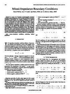
To gain understanding into the matrix notation of the transformation matrix defined above, in this section, the specific exfor a particular polynomial extension technique pression of is analyzed. This is a generalization of some techniques, which includes replication at the boundaries, linear extrapolation, and quadratic extrapolation [11]. Unlike symmetric extension, the advantage of polynomial extension is that it avoids the appearance of artificial discontinuities at the boundaries neither in the extended signal nor in its derivatives. This prevents the appearance of spurious high frequencies in each subband; therefore, we consider it to be a smooth extension. The underlying idea consists of fitting an interpolating polyto the last samples of the orignomial of degree inal signal ( ); then, this polynomial is extended to obtain . Analogously, from , which are the first samples of , we construct their corresponding interpolating polynomial and extend it to generate . Fig. 1 depicts an example of a signal extended polynomially at each edge. Note that the goal of polynomial extension is that the extended signal performs as near its edges; hence, a if the highpass filter has enough vanishing moments, processing

(9)

(10)

(13)

DOMÍNGUEZ JIMÉNEZ AND GONZÁLEZ PRELCIC: LINEAR BOUNDARY EXTENSIONS FOR FINITE LENGTH SIGNALS

3217

the new signal will not produce undesired subband coefficients of great amplitude near the edges. In our recent papers [37], we show how any new sample obtained via polynomial extrapolation on the right edge can be computed as a fixed linear combination of the previous ones; the coefficients of this linear combination are

Moreover, we have proven that the extended vector on the right , where the right extension matrix is the edge is th power of the companion matrix associated with such coef, where is obtained just ficients. In a similar way, by reversing rows and columns of . In this manner, it is a noncircular extension method associated , , and with the extension matrices . By substitution into (12) for even, we conclude that the transformation matrix associated with the polynomial extension is (14) Although the expressions of for some classical extension techniques such as zero padding, periodization, and symmetric extension can be easily deduced, they can also be found in [38]. B. Some Properties of

,

, and

To derive the main results included in Section III, we need to show some properties of , , and ; note that these matrices only depend on the prototype filters and . First of all, let us recall the following definition and notation: The subspace generated by the columns of any matrix is , called the “column subspace of ,” “image of ,” or and its dimension is the rank of the matrix . and Im are orthogonal subspaces in Lemma 1: Im of the same dimension . even Lemma 2: For (15) Besides, there are matrices , , of size such that is orthogonal, matrices , of size such is orthogonal, two invertible square matrices that , of order , and a square matrix of order such that (16)

Fig. 1. Polynomial extension of the finite signal x.

coefficients of its transfom vector . As from the is square, this is equivalent to imposing that is invert. In this section, we ible (nonsingular), and then, study the conditions under which the transformation matrix is nonsingular. A. Some Noninvertible Linear Transformation Matrices The first question arising is whether noninvertible matrices exist. In effect, the invertibility condition appears as a necessary assumption in the previous works [26], [28], [34] expressed in different but equivalent ways. In [33], an example of a noninvertible matrix was given; nevertheless, some authors [33], [39] conjecture that is always invertible whenever it is associated with linear extensions and prototype filters of equal length, but in the next theorem, we will give a family of counterexamples to this belief; moreover, for any paraunitary filterbank (constructed from filters of equal length ), we build infinitely many associated transformation matrices that are noninvertible. This constitutes a clear counterexample to the assumption presented in [33]. Theorem 1: For any two-channel cell constructed from orthogonal prototype filters of the same length, there is an infinite number of linear extensions which yield noninvertible transforms . Proof: Lemma 1 implies that any vector in is the sum of two orthogonal vectors: one and another in . In other words, any vector in can be written as a (nonunique) linear combination of the columns of and . If we apply this to any column vector of , we obtain an infinite number of matrices , such that . If is even, we build a family of transfor, , mations by taking the extension matrices null; regardless the rest of the extension matrices, the and first rows of the matrix , which are defined by (12), are

The proofs for Lemmas 1 and 2 can be found in Appendixes A and B, respectively. III. INVERTIBILITY PROBLEM Our aim is to guarantee that for a given extension, the whole transform is nonexpansive, that is, invertible. In other words, we would like to recover the samples of the original signal

Notice that all the columns depend linearly on the columns of ; , and the rank of the therefore, the rank of this submatrix is whole matrix cannot be maximum; therefore, is singular. If is odd, another column from would appear; therefore,

3218

IEEE TRANSACTIONS ON SIGNAL PROCESSING, VOL. 52, NO. 11, NOVEMBER 2004

the rank of the submatrix would be at most. Among its rows, at most are independent. Note that , . Thus, if , does and the equality is verified only if not present maximum rank; in other words, there exist infinite extension matrices that lead to noninvertible transforms . , corresponding to orthogonal We finally study the case (and ); we have that filters of length

The orthogonality condition (3) guarantees that the first column of is proportional to the vector , and the second one is pro. By taking the left extenportional to so that and , null, the sion matrices as the number first rows of form the submatrix of rank 1, which is not maximum either. We must also point out that different linear extensions may lead to the same transformation matrix . For instance, by taking the extension matrices , , we obtain the transformation matrix associated with zero padding (also generated using ). Despite this statement, we have just proven that for any paraunitary filterbank, there are always infinitely many different noninvertible transforms . B. Invertibility Criteria Once we have shown that not every matrix is invertible, we will provide some criteria that will help us analyze the invertibility of any given matrix . Obviously, is nonsingular whenever its determinant is nonzero or whenever its rank is maximum, but the order of these matrices is quite big ( ); therefore, we are interested in finding necessary and sufficient conditions which involve submatrices of smaller size so that they are easy to apply. We have obtained several criteria, which only , , and depend on the submatrices , , , of maximum order , independently of the value . Note that most of the criteria in the literature [28], [29], [39] only involve noncircular extension methods, that is, techniques where the samples appended at each edge are defined just by means of the original samples at the same edge and do not depend at all on the original samples at the other boundary. Instead, we will address the most generalized case. In our main result included below, we use the notation introduced in Section II. is independent from the Theorem 2: The invertibility of , . Moreover, is invertible central extension matrices if and only if the submatrix

(17)

has the maximum rank ( ). The proof of this result [35] is a direct consequence of the reconstruction algorithm that will be presented in Section III-C. The submatrix does not involve the central extension matrices , ; therefore, they do not affect the invertibility of .

Although they have not been included in this paper, we have found other characterizations [35], [37], [38] that require lower complexity computations for the evaluation of the invertibility . of 1) Analysis of the Polynomial Extension: The invertibility criterium so derived can be used to analyze the invertible character of a transformation matrix associated with any extension method. In particular, we consider here the polynomial extension defined in Section II-A. Theorem 3: If is a highpass filter of length with at least even vanishing moments, then polynomial extension yields an invertible transform characterized by the matrix defined in (14). In other words, polynomial extension is a nonexpansive technique whenever the prototype filter has a minimum number of vanishing moments. The proof of this theorem can be found in Appendix C. We must remark that it is the first smooth extension technique whose invertibility has been proven when using paraunitary filterbanks. As a consequence of this theorem, polynomial extenborder filters: As we will see in sion yields a family of first and last rows of contain, Section VI, the respectively, the left and right analysis biorthogonal boundary biorthogonal border filters filters. In [30], a similar set of filters, was given, but we have just proved that by using only PR is also achieved. C. Reconstruction Algorithm In this section, we propose an algorithm to perfectly recon, where is obtained from (10). Alstruct from though some algorithms have already been proposed [26], [28], [33], they only apply to noncircular extension methods. We now propose a general reconstruction algorithm that is valid for the whole set of nonsingular matrices . , it is not necessary to invert In order to recover the whole matrix ; in fact, as the system to be solved is (18) where contains the central columns of the submatrix constructed from the first and last of

, and is columns

(19)

it can be shown that two steps:

can be reconstructed block by block in

(20) (21) where

is the pseudoinverse of .

DOMÍNGUEZ JIMÉNEZ AND GONZÁLEZ PRELCIC: LINEAR BOUNDARY EXTENSIONS FOR FINITE LENGTH SIGNALS

3219

To prove (20), we can write

where ; if we multiply by , which is obtained as indicated in Section II, and taking into account (6) for , we can conclude that

This means that the first central samples can be uniquely . Moreover, as the rows of , disrecovered as played in (5), contain the synthesis filters and their even shifts, can be obviously obtained from the convolution of and these filters. To reach (21), we just reorder the system in (18): (22) which has only one solution if and only if the rank of is equal to its number of columns. Note that this reconstruction is possible if and only if (or ) presents the maximum rank ( ); therefore, this additionally constitutes the previously mentioned proof of Theorem 2. , Let us also recall that the central extension matrices do not affect the invertibility of ; thus, for the rest of this section, we will consider them to be null matrices, as occurs for all traditional extension techniques. Under this assumption, we and have that

Next, let us prove that is the null matrix so that the previous expression can be simplified. Although this result had already been intuitively proposed in [26], we now give a rigorous proof of the same. We take into account that contains the first and last columns of , and recall (6) and (9) for :

Fig. 2. Reconstruction of the central part and the edges of the original signal.

central columns of are null [see However, since the (19)], the product is equal to the product of the first and last columns of by the first and last elements and , respectively. Therefore, of , which are denoted as we can summarize the reconstruction algorithm in the following independent steps, using the matrix :

In this way, we have proven that the central samples of the original signal can be obtained from the convolution of the transform signal with the synthesis filters, whereas, if the central extension matrices are null, the border samples can be independently recovered from the borders of the transform signal, as illustrated in Fig. 2. IV. DESIGN OF NONEXPANSIVE INVERTIBLE TRANSFORMS In the last section, some criteria for analyzing the invertible character of a given extension technique have been proposed. Now, we face the problem of obtaining the explicit expression of all nonexpansive extension methods; in other words, our aim is to parameterize all the extension matrices that define invertible transforms . This way, we would get the family of all extension methods that guarantee PR property. The next result [40] shows that infinitely many invertible transformation matrices can be defined; in fact, this theorem gives a method for designing all of them (for the sake of simplicity, from now on, we will consider even). Theorem 4: is invertible if and only if there exist matrices , , , of order and an invertible matrix of order

such that

(23)

Hence, , which finalizes the proof thereof. From the last result, we have that

This result provides not only a characterization for nonexpansive transforms but also the most generalized method for their design. In order to build , it suffices to choose any invertible matrix and four matrices , , , and and introduce them into (23). Proof of this can be found in Appendix D. Up to this point, all nonexpansive extension techniques have already been designed. Now, we are going to focus

3220

IEEE TRANSACTIONS ON SIGNAL PROCESSING, VOL. 52, NO. 11, NOVEMBER 2004

on the particular case of noncircular extensions. Noncircular extensions are used most frequently, since they easily define the artificial samples as linear combinations of the adjacent original samples. This is an advantage for real-time applications, where it is desirable to process each edge independently. Apart from polynomial extension (defined in Section II-A and analyzed in Section III-B1), we wonder whether there are any other noncircular nonexpansive extension techniques. The next corollary gives us the answer: For any paraunitary filterbank, there is an infinite number of noncircular extensions that yield PR; moreover, the general parameterization of all these noncircular nonexpansive extensions is obtained. Corollary 1: A noncircular extension technique is nonexpansive if and only if there are invertible matrices , of order and two arbitrary matrices , of order such that

(24) Proof of this is straightforward: The extension is noncircular whenever , , , and in Theorem 4 are null matrices; therefore, the invertibility of only depends on the invertibility of both and . V. DESIGN OF ORTHOGONAL TRANSFORMS Having studied the extensions that lead to invertible transforms in depth, we will now focus on the ones associated to orthogonal transforms. Recall that the only extension method mentioned in the literature that preserves orthogonality is the well-known periodization technique; for that reason, we have studied the existence of other orthogonal transforms. In Appendix D, we also prove that there are infinitely many, and all of them can be obtained by means of the following result [40]. is orthogonal if Theorem 5: The transformation matrix and are null, and only if the central extension matrices and there is a unitary matrix

of order

such

that

(25)

This constitutes not only a characterization for orthogonal matrices but the most generalized method for designing any orthogonal transform as well. It suffices to choose an orthogonal matrix and introduce it into the expressions (25), which involve some matrices that were defined in Section II. As any paramorthogonal matrix of order is defined by degrees of freedom for constructing eters, there are . In our research, we have also gone a step further: the design of noncircular orthogonal extensions [41]. As periodization technique is an orthogonal circular extension, we wonder whether any noncircular orthogonal extensions exist. To this aim, and taking advantage of the general result of Theorem 5, we have achieved the first method for the design of orthogonal noncircular extensions:

is an orthogonal matrix and any of the Corollary 2: If , is null, then the other one must be null. matrices is orthogonal if and only if Moreover, a noncircular matrix there exist orthogonal matrices , of order such that

In this way, we prove that there is an infinite number of such orthogonal noncircular extensions, and there are degrees of freedom for designing them. A. Design of Smooth Adaptive Orthogonal Transforms Our final aim is to construct an extension that, like periodization, yields an orthogonal transform, but which, in contrast to periodization, does not introduce high amplitude coefficients at the boundaries of each subband in the transform domain. In other words, we would like the transform coefficients appended to the edges of each subband to be of the same magnitude as the adjacent coefficients at the center of the subband. Unfortunately, our tests show that the transform matrix associated with polynomial extension, although invertible, is not unitary. Moreover, the magnitude of the samples of a polynomial may increase excessively. Thus, as an alternative technique, we suggest the use of linear prediction-based extension. The linear prediction-based extension is defined as follows: Each appended sample is computed as a linear combination of the adjacent ones, whose coefficients are the components of of the original signal. the linear prediction vector of order This technique intuitively fulfils the smoothness property, but neither does it lead to an orthogonal transform, nor has its invertibility been demonstrated. Despite this drawback, we propose linear prediction as our target smooth extension. In other words, we assume that the samples extended by linear prediction preserve the magnitude order and search the orthogonal extension that best approximates it. Taking into account that one can define the approximation error in many different ways, we have obtained three specific approaches to the orthogonal solution [38], [42], [43]. In this section, we briefly explain our third approach, which leads to the best experimental results: The original signal is first processed via the filterbank, and then, the transform vector is extended by linear prediction in each subband, obtaining in this way the corresponding target smooth vector. As our interest is focused on the performance of the coefficients in the transform domain rather than in the time domain, the definition of this target vector perfectly matches our intuitive idea of smooth vector. Considering an original signal , the solution of the problem that we have just formulated is achieved in three steps. 1) Compute the length vector by processing through the analysis filterbank. 2) Consider each subband of (lowpass branch and highsamples pass branch), and extend each one of the per border by linear prediction. The extended vector is deof length . noted that mini3) Find an th-order orthogonal transform . mizes the error

DOMÍNGUEZ JIMÉNEZ AND GONZÁLEZ PRELCIC: LINEAR BOUNDARY EXTENSIONS FOR FINITE LENGTH SIGNALS

3221

The solution is next given in a closed form; see [43] for more , , respectively, denote the first and last details. If , be the linear prediction extension components of , let matrices of order such that (a)

Then, by simply defining the vectors

we finally obtain that the minimum error is and it is reached by any unitary matrix of order

, such that (b)

(26) Thus, it suffices to build this unitary matrix —for instance, as a Householder symmetry [44]—and substitute it in (25); the given by (12) is the orthogonal one for associated matrix is minimum. which the error Let us finally remark that there is an infinite number of unitary that verify (26), and therefore, there are infinitely matrices many orthogonal smooth transforms , all adapted to the original signal . Nevertheless, all of them provide the same smooth transform vector .

(c)

B. Experimental Results Some of the results that illustrate the good performance of our method are shown in Fig. 3. The first test signal corresponds to the cubic spline depicted in Fig. 3(a). Considering Daubechies filters of length 10 as prototype filters, the output of the two channel cell obtained using periodization is displayed in Fig. 3(b); in Fig. 3(c), we can observe the transform vector obtained by means of the optimized orthogonal boundary filters designed in [36]; Fig. 3(d) shows the transform vector using the orthogonal extension method proposed in [42], whereas Fig. 3(e) corresponds to the smooth orthogonal extension proposed in this paper. It can be clearly observed that no artificial discontinuities appear when using our smooth orthogonal techniques, neither at the borders of the lowpass branch nor in the highpass branch. On the other hand, the output vector obtained via optimized orthogonal boundary filters presents good performance only in the highpass branch but not at the borders of the lowpass branch. In this example, we conclude that our smooth orthogonal extension methods provide the best results. A more realistic signal, corresponding to an audio frame, is shown in Fig. 4(a). Considering length 26 Daubechies filters, in Fig. 4(b), we display the transform vectors obtained through periodization, our smooth orthogonal extension algorithms, and the optimized boundary filters presented in [36]. These four vectors only differ at the borders of both subbands so it suffices to compare such border coefficients in Fig. 4(b). It is clear that the performance of the periodic extension method is overcome by the rest of the orthogonal techniques; but in this case, we also observe that the output of the new algorithm presents highpass coefficients of smaller magnitude than the one presented in [42] and lowpass coefficients of smaller magnitude than the ones obtained through the algorithm described in [36]. This means that

(d)

(e) Fig. 3. (a) Original cubic signal. (b) Transform vector using periodization. (c) Output vector by using the optimized orthogonal boundary filters. (d) Transform vector by means of the existing smooth orthogonal extension technique. (e) Output vector by means of the proposed smooth orthogonal extension method.

the new smooth orthogonal technique presents the best performance in the transform domain. VI. BOUNDARY FILTERS DESIGN VERSUS BOUNDARY EXTENSION METHODS To finish our work, we compare our theoretical formulation of signal extension techniques to the boundary filters design in order to determine the relationship between both approaches and the advantages of each method. Techniques for the design of biorthogonal and orthogonal boundary filters have been proposed in the literature [31], [32]. Although signal extension techniques constitute an older solution to the problem of boundary treatment and one could initially think that the direct design of border filters is a completely independent approach, it can be easily shown that both types of techniques lead to transformation matrices with with a common expression. Thus, we can compare matrix

3222

IEEE TRANSACTIONS ON SIGNAL PROCESSING, VOL. 52, NO. 11, NOVEMBER 2004

where the rows of and , respectively, contain the left right boundary filters. Note that and share their and central rows since they contain the prototype filters , , and their even shifts. Hence, any nonexpansive extension method yields a set of biorthogonal boundary filters, which are contained in the first and the last rows of the matrix given in (11):

Biorthogonal boundary filters designed by means of the algorithm given in [32] are of the form

where , 2 ,3, and 4 have size . They are dehave independent rows; they contain signed so that and nonzero initial coboundary filters with at most efficients and nonzero final coefficients. Note that central components that these boundary filters have are null so that the equation above does not constitute the most generalized expression for biorthogonal boundary filters. On the other hand, by using any extension method, we observe that the boundary filters that appear in the first and last rows of do not present the most generalized expression either (for instance, the upper right corner must be of the form ). Nevertheless, as is nonsingular, linear algebra assures that any other matrix containing boundary filters and the same prototype filters in its rows can be written as (27) Therefore, and contain left and right biorthogonal is nonsingular) if and only if the boundary filters (that is, matrix

Fig. 4. (a) Original audio frame. (b) Solid line: Central subband samples of the transform vector, common to all the studied techniques; coefficients at the borders of each subband obtained by means of periodization (represented by circles), the optimized orthogonal boundary filter design technique (marked with crosses), the existing smooth orthogonal transform (depicted as squares), and the proposed algorithm (triangles). (c) Detail of the border coefficients in the lowpass band. (d) Detail of the border coefficients for the highpass band.

matrix , corresponding to the transform associated with the use of any set of boundary filters:

is invertible of order

. In other words,

any general set of boundary filters may be designed via a nonsingular matrix by means of (27). In some applications, it is desirable to work with short boundary filters. Herley’s algorithm [32] provides all biorthognonzero coefficients. By onal boundary filters with at most even), we can also derive a new means of our results (for design method for all of the boundary filters of this type. • Recalling Theorem 4, we build a nonexpansive noncircular matrix : It suffices to choose two invertible ma, of order and two arbitrary matrices trices , of order and substitute them into (24) and (12) to get

Its first rows contain the biorthogonal left boundary filters of at most nonzero coefficients, as well as the biorthogonal right boundary filters that appear in its last rows. As is invertible, any other set of biorthogonal boundary filters can be written as in (27).

DOMÍNGUEZ JIMÉNEZ AND GONZÁLEZ PRELCIC: LINEAR BOUNDARY EXTENSIONS FOR FINITE LENGTH SIGNALS

3223

TABLE I COMPLEXITY OF THE DESIGN METHOD

• Next, it suffices to impose that the final columns columns of be null in (27). of and the first Algebraic manipulations lead us to state that and must be null, and , must be of the form

being arbitrary matrices. • Finally, we make the matrix product (27) by denoting

This way, we summarize the proposed design method. Theorem 6: When using the paraunitary two-channel filter, any set of left and bank given by and of length can right biorthogonal boundary filters of maximum length always be written as (28)

are null. In other words, the general set of orthogonal boundary of order filters may be designed by fixing a unitary matrix , substituting it in (25) in order to obtain the orthogonal matrix , and applying (27). Note that our design method is the most generalized one, because the traditional algorithm proposed in [31] only pro. For vides orthogonal boundary filters of maximum length instance, the orthogonal boundary filters associated with periodization are not included in that approach. Instead, our method considers both circular and noncircular extensions, leading to all the possible kinds of orthogonal boundary filters. Anyway, let us show how our method can also be used to design the specific set of short orthogonal boundary filters of a . In doing this, we will be able to maximum length of, say, compare it with the traditional boundary filter design algorithm. To this end, it suffices to modify Theorem 6 to the orthogonal case, obtaining the following result. Theorem 7: When using a paraunitary two-channel filter( even), any set of associated bank of length left and right orthogonal boundary filters of maximum length can be always written as

(29) where we have the following. 1) and are extension matrices satisfying the invertibility condition for noncircular extensions, that is, they are defined by (24) by choosing two invertible matrices and and two arbitrary matrices , of order . and are nonsingular matrices of order . 2) and are arbitrary matrices of size . 3) The expressions given in (28) and (29) are the most gener, alized ones for left and right boundary filters of length respectively. It suffices to follow the three steps in order to construct all of them. Unlike in the traditional design algorithm [32], there is no need to use any iterative orthogonalization procedure; the main advantage of the proposed design method is that the solution is given in a closed form. A. Orthogonal Boundary Filters Design Finally, in this section, we consider the specific family of orthogonal boundary filters associated with signal extension techniques and compare our design method to the traditional algorithm for the design of orthogonal boundary filters [31]. First of all, we take advantage of our proposed method for the design of biorthogonal boundary filters by just applying the orthogonality property. In effect, given a paraunitary filterbank, any set of orthogonal boundary filters appear in the first and last rows of any matrix of the form (27) whenever is orthogonal,

is unitary of order

, and

and

where and are orthogonal extension matrices defined through Corollary 2—just by choosing two unitary matrices , of order —and , are unitary matrices of order . Once we have presented our design method for short orthogonal boundary filters, we compare it with the traditional algorithm of [31]. • On the one hand, note that the proposed method is very easy to implement, and, unlike the traditional one, it does not need any iterative procedure since the solution is given in a closed form. • On the other hand, our method only involves premultiplication by unitary matrices, so numerically, it performs well. • Finally, we compare their computational complexities, measured as the number of multiplications. The proposed algorithm involves a first step (construction of the basic , , , , , , and , which only matrices depend on the prototype filters, and can be computed once and for all), a second step (the extension design itself, by , ), and the third step (premultiplication means of , ). Table I shows the computational by matrices . cost of each step and the total cost of order In contrast, the computational cost for the traditional , algorithm has been proved [41] to be of order even if the algorithm converges in the minimum number of iterations. We conclude that our method is at least four times faster than the border filter design algorithm.

3224

IEEE TRANSACTIONS ON SIGNAL PROCESSING, VOL. 52, NO. 11, NOVEMBER 2004

For all these reasons, we conclude that the design method presented here constitutes a clear improvement to the orthogonal border filters approach. VII. CONCLUSIONS AND FURTHER WORK Artificial extension methods that lead to invertible transforms can be designed efficiently. An appropriate matrix formulation of size-limited paraunitary filterbanks allows us to obtain a novel operator for the study of boundary extension techniques. Criteria for the analysis of the invertibility of the transformation matrix, that is, the biorthogonality of the boundary filters corresponding to a given extension, are also introduced. New algorithms are developed for the efficient design of all extensions that generate both nonsingular and orthogonal transforms. In addition to new solutions, the constructions obtained by means of our algorithm also include all the designs generated with previously proposed techniques. The results presented here constitute an indispensable piece for the study of extensions with additional properties, which become an interesting alternative to symmetric extension or periodization when using paraunitary filterbanks. In this respect, we have addressed the problem of designing extensions or boundary filters that do not introduce artificial discontinuities: On the one hand, polynomial extension is a smooth technique whose PR property has been demonstrated; on the other hand, we have achieved the design of smooth adaptive orthogonal extensions. The optimal transformation matrix and the smooth transform vector are determined explicitly. The absence of artificial discontinuities in the transform domain is clear from our tests, overcoming the main drawback of existing orthogonal signal extension methods. Finally, our theoretical formulation also provides general techniques for the design of biorthogonal and orthogonal boundary filters that constitute interesting contributions to border filter theory. The main issue of our current research is the design of nonadaptive smooth orthogonal boundary filters that are valid for a wide variety of signals.

Second, the orthogonality condition (4) guarantees that ; this means that Im and Im are orthog. As the sum of their dimensions is at onal subspaces in [because ], we least the dimension of and Im are orthogonal complementary derive that subspaces in . odd However, is a submatrix of , and they share their columns, which we have just proven to be linearly independent, , and we derive that so both of them present rank . Similarly, Im Im , and we conclude that and Im are orthogonal complementary subspaces in Im (of the same dimension ). APPENDIX B PROOF OF LEMMA 2 Matrix ular, for

has orthonormal rows; in partic, we have that

has orthonormal rows; therefore, ; this guarantees the identities in (15). For the second part of the lemma, recall Lemma 1: The row and are orthogonal, and their dimension subspaces of is . We build respective orthonormal bases of each row subspace (for instance, by means of a Gram–Schmidt orthogoand nalization procedure [44]); thus, we get matrices whose rows contain, respectively, orthonormal row bases of and . Second, by repeating the orthogonalization process and , we obtain matrices over the columns of and with orthonormal columns; this guarantees the factorizations of and in i) of (16) and ii) of (16). In order to prove the identity iii) of (16), we use (which has just been demonstrated); this means that such that , but there must be a matrix it is also equivalent to any of the following expressions:

APPENDIX A PROOF OF LEMMA 1 First of all, note that we can also write , where , are square submatrices of order :

.. .

..

.. .

..

.

..

.

.

..

..

.

..

.

.

As they appear in echelon form, and and not null matrices, the ranks .

In addition, matrix

is orthogonal; therefore, , and we finally obtain

.. .

..

.

..

. and

APPENDIX C PROOF OF THEOREM 3 .. . [see (2)] are are then at least

, we observe that it is invertBy applying Theorem 2 to ible if and only if . In other words, it is necessary and sufficient that the null space of the matrices and is zero. Let us consider any vector such that ; our aim is to show that is zero.

DOMÍNGUEZ JIMÉNEZ AND GONZÁLEZ PRELCIC: LINEAR BOUNDARY EXTENSIONS FOR FINITE LENGTH SIGNALS

Considering the samples of the signal , we extraposamples per border in a polylate this vector by appending . This way, is a discrete polynomial nomial way to form of degree ; we process it by means of the two-channel cell and obtain

We have applied the fact that and the assumption . As is a polynomial , the hypothesis about the vansequence of degree ishing moments guarantees that the even components of (say, ) are zero. In particular, the the highpass coefficients of central even components of are the even elements of , which must be zero, but the even rows of are linearly independent and generate the rest of the rows; theremust be null; moreover, this fore, the whole vector means that we can write for some vector . Then, the last components of are , where we have used that , which is a consequence of iii) of has null even (16). Thus, we have another vector such that components; therefore, it must be identically zero for the same reason. We summarize that

In other words, not only the highpass coefficients of the are zero, but so are its last lowpass coeffipolynomial cients. Recall that the lowpass components form another , but it has more roots than its depolynomial of degree gree; therefore, it must be the null polynomial. We conclude that . Finally, by computing , we derive that must be null. Analogously, we would show that , finishing the proof. APPENDIX D PROOF OF THEOREM 4

(30) ,

, and

By substituting the identities for , , and given in (16), in the expression (17) for , it is easy to show that this matrix , where can also be written as

Note that is orthogonal and that has orthonormal columns. Thus, presents maximum rank if and only if presents maximum rank; this happens whenever

is invertible. This way, we can write , , 2, 3, and 4 by ( , 2, 3, and 4) and introduce them in (30) in means of order to finally obtain the identities in (23) of the theorem. APPENDIX E PROOF OF THEOREM 5 We first check that a necessary condition for to be orthogand are null; in effect, the onal is that central columns of , given by (11), form the submatrix , where

.. .

..

.

..

.

..

.

..

.

..

.

.. . .. . .. .

Equation (15) implies that and that null. Thus, has orthonormal columns if and only if

From Theorem 2, has an inverse if and only if presents maximum rank ( ). On the other hand, by using the orthogoand and and , the nality conditions of matrices extension matrices verify that

where matrices . order

3225

, 2, 3, and 4 are square of

is

Therefore, must be null, as well as and . Hence, it suffices to study the orthogonality of matrices of the type (12). In this case, we note that is orthogonal if and only if the columns of its submatrix (or ) are orthonormal. Now, by recalling the steps of the demonstration given in so that contains orAppendix D, we can write does. By using the identities thonormal columns whenever (15) and (16), we finally deduce that this happens if and only if ( , 2, 3, and 4) are null, and is unitary, which finishes the proof.

3226

IEEE TRANSACTIONS ON SIGNAL PROCESSING, VOL. 52, NO. 11, NOVEMBER 2004

REFERENCES [1] P. P. Vaidyanathan, “Multirate digital filters, filterbanks, polyphase networks, and applications: A tutorial,” Proc. IEEE, vol. 78, pp. 56–93, Jan. 1990. [2] A. N. Akansu and R. A. Haddad, Multiresolution Signal Decomposition. San Diego, CA: Academic, 1992. [3] C. Herley and M. Vetterli, “Wavelets and filterbanks: Theory and design,” IEEE Trans. Signal Processing, vol. 40, pp. 2207–2232, Sept. 1992. [4] A. K. Soman and P. P. Vaidyanathan, “On orthonormal wavelets and paraunitary filterbanks,” IEEE Trans. Signal Processing, vol. 41, pp. 1170–1183, Mar. 1993. [5] P. P. Vaidyanathan, Multirate Systems and filterbanks. Englewood Cliffs, NJ: Prentice-Hall, 1993. [6] S. G. Mallat, “A theory for multiresolution signal decomposition: The wavelet representation,” IEEE Trans. Pattern Anal. Machine Intell., vol. 11, pp. 674–693, July 1989. [7] I. Daubechies, Ten Lectures on Wavelets. Philadelphia, PA: SIAM, 1992. [8] C. Herley, J. Kovacevic, K. Ramchandran, and M. Vetterli, “Tilings of the time-frequency plane: Construction of arbitrary orthogonal bases and fast tiling algorithms,” IEEE Trans. Signal Processing, vol. 41, pp. 3341–3359, Dec. 1993. [9] M. V. Wickerhauser, Adapted Wavelet Analysis From Theory to Software. Wellesley, MA: AK Peters, 1994. [10] M. Vetterli and J. Kovacevic, Wavelets and Subband Coding. Englewood Cliffs, NJ: Prentice-Hall, 1995. [11] G. Strang and T. Q. Nguyen, Wavelets and Filterbanks. Wellesley, MA: Wellesley-Cambridge, 1996. [12] A. N. Akansu and M. J. T. Smith, Subband and Wavelet Transforms: Design and Applications. Boston, MA: Kluwer Academic, 1996. [13] C. S. Burrus, R. A. Gopinath, and H. Guo, Wavelets and Wavelet Transforms. Upper Saddle River, NJ: Prentice-Hall, 1997. [14] A. R. Lindsey, “Wavelet packet modulation for orthogonally multiplexed communication,” IEEE Trans. Signal Processing, vol. 45, pp. 1336–1339, May 1997. [15] A. N. Akansu, P. Duhamel, X. Lin, and M. de Courville, “Orthogonal transmultiplexers in communication: A review,” IEEE Trans. Signal Processing, vol. 46, pp. 979–995, Apr. 1998. [16] L. Vandendorpe et al., “Fractionally spaced linear and decision-feedback detectors for transmultiplexers,” IEEE Trans. Signal Processing, vol. 46, pp. 996–1011, Apr. 1998. [17] Y. Shiyou et al., “Wavelet-Galerkin method for computations of electromagnetic fields,” IEEE Trans. Magn., vol. 34, pp. 2493–2496, Sept. 1998. [18] G. B. Giannakis, “Highlights of signal processing for communications,” IEEE Signal Processing Mag., vol. 16, pp. 14–50, Mar. 1999. [19] A. Scaglione, G. B. Giannakis, and S. Barbarossa, “Redundant filterbank precoders and equalizers—Part I: Unification and optimal designs,” IEEE Trans. Signal Processing, vol. 47, pp. 1988–2006, July 1999. [20] T. Painter and A. Spanias, “Perceptual coding of digital audio,” Proc. IEEE, vol. 88, pp. 451–515, Apr. 2000. [21] D. S. Taubman and M. W. Marcellin, Jpeg2000: Image Compression Fundamentals, Standards, and Practice. Boston, MA: Kluwer, 2001. [22] N. G. Prelcic, F. P. González, and M. E. D. Jiménez, “Wavelet-packetbased subband adaptive equalization,” Signal Process., vol. 81, pp. 1641–1662, Aug. 2001. [23] P. P. Vaidyanathan, Y. Lin, S. Akkarakaran, and S. Phoong, “Discrete multitone modulation with principal component filterbanks,” IEEE Trans. Circuits Syst. I, vol. 49, pp. 1397–1412, Oct. 2002. [24] W. E. Hutchcraft and R. K. Gordon, “Two-dimensional higher order wavelet-like basis functions in the finite element method,” in Proc. 34th Southeastern Symp. System Theory, Huntsville, AL, Mar. 2002, pp. 147–151. [25] G. Karlsson and M. Vetterli, “Extension of finite length signals for subband coding,” Signal Process., vol. 17, pp. 161–168, June 1989. [26] R. L. de Queiroz, “Subband processing of finite-length signals without border distortions,” in Proc. IEEE ICASSP, vol. 4, San Francisco, CA, Mar. 1992, pp. 613–616. [27] R. H. Bamberger, S. L. Eddins, and V. Nuri, “Generalized symmetric extension for size-limited multirate filterbanks,” IEEE Trans. Image Processing, vol. 3, pp. 82–87, Jan. 1994. [28] J. N. Bradley and V. Faber, “Perfect reconstruction with citically sampled filterbanks and linear boundary conditions,” IEEE Trans. Signal Processing, vol. 43, pp. 994–997, Apr. 1995. [29] R. L. de Queiroz and K. R. Rao, “On reconstruction methods for processing finite-length signals with paraunitary filterbanks,” IEEE Trans. Signal Processing, vol. 43, pp. 2407–2410, Oct. 1995.

[30] A. Cohen, I. Daubechies, and P. Vial, “Wavelets on the interval and fast wavelet transforms,” Applied Comput. Harmon. Anal., vol. 1, pp. 54–81, Jan. 1993. [31] C. Herley and M. Vetterli, “Orthogonal time-varying filterbanks and wavelet packets,” IEEE Trans. Signal Processing, vol. 42, pp. 2650–2663, Oct. 1994. [32] C. Herley, “Boundary filters for finite-length signals and time-varying filterbanks,” IEEE Trans. Circuits Syst. II, vol. 42, pp. 102–114, Feb. 1995. [33] R. L. de Queiroz, “Further results on reconstruction methods for processing finite-length signals with perfect reconstruction filterbanks,” IEEE Trans. Signal Processing, vol. 48, pp. 1814–1816, June 2000. [34] V. Silva and L. de Sá, “General method for perfect reconstruction subband processing of finite length signals using linear extensions,” IEEE Trans. Signal Processing, vol. 47, pp. 2572–2575, Oct. 1999. [35] M. E. Dominguez Jiménez and N. G. Prelcic, “Processing finite length signals via filterbanks without border distortions: A nonexpansionist solution,” in Proc. IEEE ICASSP, vol. 3, Phoenix, AZ, Mar. 1999, pp. 1481–1484. [36] A. Mertins, “Boundary filter optimization for segmentation-based subband coding,” IEEE Trans. Signal Processing, vol. 49, pp. 1718–1727, Aug. 2001. [37] M. E. Dominguez Jiménez and N. G. Prelcic, “Polynomial extension method for size-limited paraunitary filterbanks,” in Proc. Eur. Signal Process. Conf., vol. 2, Toulouse, France, Sept. 2002, pp. 545–548. [38] M. E. Dominguez Jiménez, “Diseño de Extensiones Para Procesamiento de Señales Finitas Mediante Wavelets,” Ph.D. dissertation, Univ. Politécnica Madrid, Madrid, Spain, 2001. [39] J. Williams and K. Amaratunga, “A discrete wavelet transform without edge effects using wavelet extrapolation,” J. Fourier Anal. Applicat., vol. 3, no. 4, pp. 435–449, 1997. [40] M. E. Dominguez Jiménez and N. G. Prelcic, “Design of nonexpansionist and orthogonal extension methods for tree-structured filterbanks,” in Proc. IEEE ICASSP, vol. 1, Istanbul, Turkey, June 2000, pp. 532–535. , “New orthogonal extension methods for tree-structured filter[41] banks,” in Proc. Eur. Signal Process. Conf., vol. 2, Tampere, Finland, Sept. 2000, pp. 1073–1076. , “Orthogonal extensions of AR processes without artificial discon[42] tinuities for size-limited filterbanks,” in Proc. IEEE Workshop Statistical Signal Process., Singapore, Aug. 2001, pp. 579–582. , “Smooth orthogonal signal extensions for paraunitary tree-struc[43] tured filterbanks,” in Proc. IEEE ICASSP, vol. 2, Orlando, FL, May 2002, pp. 1233–1236. [44] G. H. Golub and C. F. Van Loan, Matrix Computations, Third ed. Baltimore, MD: Johns Hopkins Univ. Press, 1996.

María Elena Domínguez Jiménez was born in Madrid, Spain, in 1969. She received the degree in mathematical sciences from the Universidad Complutense de Madrid in 1992 and the Ph.D. degree from the Universidad Politécnica de Madrid in 2001. Since 1992, she has been an assistant professor at the Departamento de Matemática Aplicada, E.T.S.I. Industriales, Universidad Politécnica de Madrid. Her research interests include audio compression, multiresolution signal processing, wavelets, and filterbank theory. Dr. Domínguez received an Extraordinary Award from the Universidad Politécnica de Madrid for the best doctoral dissertation in 2002 .

Nuria González Prelcic (M’99) was born in Vigo, Spain, in 1970. She received the B.E. and Ph.D. degrees in telecommunications engineering from the Universidad de Vigo in 1993 and 1998, respectively. She is currently an Associate Professor with the Departamento de Teoría y las Comunicaciones, Universidad de Vigo. Her interests lie in the areas of wavelets and filterbanks and digital signal processing applied to communications.