Linear Image Registration through MRF Optimization - CAMP@TUM

LINEAR IMAGE REGISTRATION THROUGH MRF OPTIMIZATION Ben Glocker1,2 , Darko Zikic1 , Nikos Komodakis3 , Nikos Paragios2,4 , Nassir Navab1 1

Computer Aided Medical Procedures (CAMP), Technische Universit¨at M¨unchen, Germany 2 Laboratoire MAS, Ecole Centrale Paris, Chatenay-Malabry, France 3 Computer Science Department, University of Crete, Greece 4 Equipe GALEN, INRIA Saclay - Ile-de-France, Orsay, France

ABSTRACT We propose a Markov Random Field formulation for the linear image registration problem. Transformation parameters are represented by nodes in a fully connected graph where the edges model pairwise dependencies. Parameter estimation is then solved through iterative discrete labeling and discrete optimization while a label space refinement strategy is employed to achieve sub-millimeter accuracy. Our framework can encode any similarity measure, allows for automatic reduction of the degrees of freedom by simple changes on the MRF topology, and is robust to initialization. Promising results on real data and random studies demonstrate the potential of our approach. Index Terms— Linear Image Registration, Markov Random Fields, Discrete Optimization 1. INTRODUCTION In the last years, the solution of computer vision problems by Markov Random Fields (MRFs) [1] and discrete optimization has become increasingly popular for medical imaging applications such as segmentation [2] or non-linear registration [3]. Recent advances [4, 5] in discrete optimization methods make this approach very attractive. However, linear image registration [6, 7], which is one of the most important and basic techniques in medical image processing has not yet been solved by discrete optimization. In this paper we address this issue and present a linear registration method which formulates the problem as an MRF model and solves it by discrete optimization.

where Tˆ is the optimal transformation and ξ ia an arbitrary intensity-based similarity measure. We consider T to be a linear transformation, more precisely we will focus on affine, anisotropic similarity, and rigid transformations which are often used in medical settings. There is a wide choice of similarity measures which can be employed, ranging from the sum of squared differences (SSD) to more sophisticated statistical measures such as mutual information (MI) [8, 9]. Formulating Eq. (1) as an MRF problem has the advantage that the similarity measure is easily interchangeable, since no derivatives of the measure are required. Furthermore, discrete optimization methods have generally a large capture range. Combined with intelligent discretization strategies such methods have potential for robust image registration. In Sec. 2.1, we present the parameterization of the transformation model. Sections 2.2 and 2.3 describe our MRF model and discretization strategy and in Sec. 2.4 further features of the framework are given. 2.1. Parameterization Affine transformations in homogeneous coordinates are linear transformations which can be written in the form   ˆ  A  , (2) 0 1 where Aˆ is a 2×3 or 3×4 matrix for 2D and 3D respectively, resulting in 6 degrees of freedom (DOF) in 2D and 12 DOF in 3D. We employ a parameterization in which the affine transformation is decomposed as

2. METHOD The task of image registration is to recover a transformation T which aligns two images I, J : Ω 7→ R. A common approach for modeling this problem is by energy minimization as Tˆ = arg min ξ (I, J ◦ T ) , T

(1)

The authors gratefully acknowledge the partial support of this work by Siemens Corporate Research (SCR), Princeton, NJ, USA.

A = Mt Rφ Rθ−1Ds Rθ .

(3)

Here, Mt is a translation, Rφ is a rotation, and Rθ−1Ds Rθ represents the shearing transformation. For the shearing, Rθ is a rotation and Ds is a diagonal matrix, representing anisotropic scaling. We parameterize the single matrices of Eq. (3) by respective parameters, compare also [10]. The 3D rotation matrices are parameterized by Euler angles. The resulting pa-

tx Ãtx Á

the pairwise terms are able to model the energy resulting from a simultaneous change of two parameters. Hence, we use the pairwise potentials to model the energy corresponding to a simultaneous variation of the parameters pi and pj as

μ

Ãtx ty

ty

tx

sx

ty

sy

Ãty Á

Á

ψij (xi , xj ) = ξ (I, J ◦ Tij ) ,

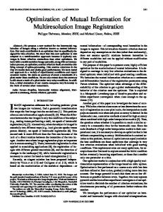
Á Fig. 1: MRF topology for 2D linear registration in case of rigid (left) and affine transformations (right).

rameter vectors for the 2D and 3D case are p = [φ, tx , ty , sx , sy , θ]

(4)

p = [φx , φy , φz , tx , ty , tz , sx , sy , sz , θx , θy , θz ] .

(5)

An advantage of this parameterization is that it can be used also for less general transformations. Rigid transformations are obtained, if D = Rθ = Id, similarity transformations are encoded for Rθ = Id.1 Similarly, pure translation, rotation, scaling, or shearing transformation, or any combination thereof can be achieved. 2.2. Markov Random Fields for Linear Registration The key idea of our approach is to reformulate parameter estimation for linear registration as a discrete labeling problem. To this end, we construct a graph G = (V, E) consisting of a set of nodes V and a set of edges E. Each node vi ∈ V corresponds to one parameter pi of the linear transformation, while an edge (vi , vj ) ∈ E between two nodes represents their dependency. For each node, we introduce a set of discrete labels Li which is associated with a quantized version of the parameter space Φi . This way, image registration becomes a labeling task where one seeks to assign an optimal label xi ∈ Li to each of the nodes such that the resulting transformation aligns the two images. A common approach for modeling discrete labeling tasks in terms of energy minimization is the usage of first-order MRFs. The general form of the MRF energy is defined by two sums over potential functions X X Emrf = ψi (xi ) + ψij (xi , xj ) , (6) vi ∈V

(vi ,vj )∈E

where ψi are the unary potentials determining the energy of assigning a label xi to a node vi , and ψij are the pairwise potentials determining the energy of assigning a pair of labels (xi , xj ) to the connected nodes vi and vj . Note that the unary potentials are modeling the energy for a single parameter independently of all others. Since the linear transformation parameters are highly dependent, unary potentials are not appropriate for their modeling. In contrast, 1 Please note that the similarity transformation includes anisotropic scaling which is important for inter-subject registration.

(7)

where the transformation Tij encodes the change in the parameters pi and pj . In order to force the global consistency of the transformation parameters, we connect all nodes between each other such that we obtain a fully connected graph G ?=(V, E ? ). Exemplary configurations for different types of linear transformations are illustrated in Fig. 1. Finally, we define the MRF energy for the linear registration problem as posed in Eq. (1) as Elinreg =

X (vi ,vj

=

ψij (xi , xj )

(8)

)∈E ?

X

ξ (I, J ◦ Tij ) .

(9)

(vi ,vj )∈E ?

In the literature, many optimization algorithms exist for efficiently solving discrete labeling problems in form of an MRF. We use a recently proposed method called FastPD [5] which has successfully been used for non-linear registration [3]. Due to the limited space, we refer the reader to the given references for more details about the optimization algorithm. In the following, we describe the important part of parameter space discretization.

2.3. Parameter Space Discretization We consider the following discretization strategy for obtaining the quantized versions Φi of the parameter space. For each parameter, we define a minimum and maximum value which determines the parameter range and perform a uniform sampling of the range. Here, the number of labels plays a crucial role. A sparse sampling might result in inaccurate registration while dense sampling increases complexity. To overcome this problem, we employ a successive label space refinement. In each iteration k, we rescale the parameter range by a factor αk and compute a new MRF labeling. The successive label space refinement allows us to keep the number of labels quite small and we can start with a large parameter range, while being able to achieve sub-millimeter registration accuracy. For the computation of Eq. (7), we need to compute the ˆ ij is the varipotential transformations Tij = T (ˆ pij ), where p ation of the current parameter vector p by ∆pij at parameters pi and pj . For all parameters pˆk , except for scaling, the variation is achieved by addition, i.e. pˆk= pk+∆pk , while for the scaling parameters pˆs multiplication is used pˆs= ps ∆ps .

30

800

25 600

20 15

400

10 200 5 0

0

1

2

3

4

5

6

7

8

Fig. 2: Error distribution of the 3D affine random study test. Of the 200 trials, 3 were classified as failed with an error >10mm. The histogram of the successful trials is presented above and the distribution has a mean of 2.02mm (±0.84mm), and median of 1.88mm.

0

0

0.05

0.1

0.15

0.2

0.25

(a) Error distribution for all classes.

0.25 0.2

2.4. Further Method Features The described registration method is performed with a standard multi-scale strategy. The method also supports random subsampling strategies, which are often used to improve the runtime, cf. e.g. [11] and references therein. Furthermore, it is easy to implement a stratified approach, which is often used in real applications [12] and consists in sequentially performing registrations of increasing complexity. Due to the flexible parameterization as described in Sec.2.1, automatic reduction of the degrees of freedom is achieved by simple changes on the MRF topology. Since our method performs these modifications automatically if the search range for one parameter is set to zero, there is no need for explicit implementation of the single registration methods.

0.15 0.1 0.05 0 0

1

2

3

4

5

6

7

8

(b) Boxplot description of error for single test classes.

Fig. 3: Error distribution of the 2D affine random study test. (a) Error over all classes. Of the 7000 trials, 19 from class 7 had an error >1mm and were classified as failed. The histogram of the successful trials is presented above and the distribution has a mean of 0.05mm (±0.03mm), and median of 0.04mm. (b) The error distribution for single classes as boxplot. The mean is presented by the blue cross, the median by the green line.

3. EVALUATION We test our method by random studies in 2D and 3D on monomodal brain (Sec. 3.2, 3.1) as well as by a series of multimodal registrations (Sec. 3.3). All experiments are performed on brain data from the the Retrospective Image Registration Evaluation Project (RIRE) database. We employ a CT image with a resolution of 512×512×29 and a physical voxel size of 0.65×0.65×4mm and 3 MR images (T1,T2,PD) with a resolution of 256×256×26 and a voxel size of 1.25×1.25×4mm. The number of labels per label space Li is set to 9 and we found a fixed scaling factor of α = 2/3 to be efficient. 3.1. 3D Random Study The 3D random study is performed on a CT volume. Random affine transformations are applied to the source image, and the warped image is used as target. The transformation parameters are uniformly drawn from certain ranges. Translations result from ±10mm, rotations lie between ±20◦ , scalings range from [0.8, 1.2], and the shearing angle parameters θ are drawn from ±5◦ . We performed 200 experiments with the same parameters, which were set manually. We use a subsampling strategy with 5% of randomly chosen voxels and SSD as similarity measure. The registration error is computed as the average distance (AD) of the corner points of a centered 200mm cube, warped by the ground truth and the estimated

transformation. The results are summarized in Fig. 2. The average runtime is about 3 minutes. 3.2. 2D Random Study The 2D random study is performed on a slice from the CT image in same way as the 3D study. We additionally bin the random transformations into 7 classes of increasing complexity in order to study the capture range of the method. The classes sample the parameter space equidistantly, for translation ([0, 35]mm), rotation ([0, 42]◦ ), scaling (1±0.025 to 1± 0.175), and shearing angle ([0, 7]◦ ). For example, class 7 contains translations from [30, 35]mm, rotations from [36, 42]◦ , scalings from 1±0.175, and shearing rotation of [6, 7]◦ . The error is evaluated on the corners of a 200mm centered square. We perform 1000 tests for every single class, and evaluate the registration error for the single classes as well as the complete range in Fig. 3. The average runtime is about 20 seconds. In addition, we test the robustness w.r.t. to initialization by testing the registration for large rotations. For 1000 trials we generate targets by small translation (±10mm) and scaling (1 ± 0.1), and a large rotation ([90, 180]◦ ). In 99.3% of the cases the method successfully recovers the transformation with sufficient precision for further steps (error below 20mm).

(a) CT to MR-T1

(b) CT to MR-T2

(c) CT to MR-PD

Fig. 4: Checkerboard visualization of the multi-modal registration. The errors from left to right are 1.36, 4.20, and 2.27mm.

3.3. 3D Multi-Modal Registration Our last experiment is a multi-modal registration scenario. For all registrations, a ground truth transformation is available obtained through a fiducial landmark registration performed by the providers of the database. A CT image is registered to three MR images acquired with different protocols (T1, T2, and PD). For the tests, we use a subsampling strategy with 20% of randomly chosen voxels. We also use the stratified approach (Sec. 2.4), where translation correction is performed prior to rigid registration. Using the ground truth, we determine the error by measuring the AD for a centered cube of 334×334×112mm. The AD for the initial alignment before registration is 46.18, 56.13, and 67.61mm for T1, T2, and PD respectively. After registration the error is 1.36, 4.20, and 2.27mm. For all registrations, we use the entropy correlation coefficient (ECC) proposed in [8]. Visual results are illustrated in Fig. 4. Here, the average runtime is about 5 minutes. 4. CONCLUSION In this paper, we have derived an MRF formulation for the linear image registration problem. The transformation model is decomposed into the individual parameters which are represented by nodes in a fully connected graph. Parameter estimation is then solved through iterative discrete labeling and discrete optimization while using a label space refinement strategy and a multi-scale approach. Our framework can encode any similarity measure without need for substantial modifications and allows for stratified registration since any subclass of affine transformation can be modeled by simple changes on the MRF topology. We evaluated our method on real data and extensive random studies. We also showed that our method is robust w.r.t. initial alignment. In future work, performance comparison with other methods will be performed. Since the main computation is based on image warping and evaluation of the similarity measure, we believe that our method is especially suitable for GPU optimization.

5. REFERENCES [1] S. Geman and D. Geman, “Stochastic relaxation, gibbs distributions, and the bayesian restoration of images,” in PAMI, 1984. [2] Y.Y. Boykov and M.-P. Jolly, “Interactive graph cuts for optimal boundary & region segmentation of objects in n-d images,” in ICCV, 2001. [3] B. Glocker, N. Komodakis, G. Tziritas, N. Navab, and N. Paragios, “Dense image registration through mrfs and efficient linear programming,” Med. Im. Anal., 2008. [4] Y. Boykov, O. Veksler, and R. Zabih, “Fast approximate energy minimization via graph cuts,” in ICCV, 1999. [5] Nikos Komodakis, Georgios Tziritas, and Nikos Paragios, “Fast, approximately optimal solutions for single and dynamic mrfs,” in CVPR, 2007. [6] J.V. Hajnal, D.J. Hawkes, and D.L.G. Hill, Medical Image Registration, CRC Press, 2001. [7] B. Zitova and J. Flusser, “Image registration methods: a survey,” Image and Vision Computing, 2003. [8] F. Maes, A. Collignon, D. Vandermeulen, G. Marchal, and P. Suetens, “Multimodality image registration by maximization of mutual information,” TMI, 1997. [9] Paul Viola and William M. Wells, “Alignment by maximization of mutual information,” IJCV, 1997. [10] R. Hartley and A. Zisserman, “Multiple view geometry in computer vision,” 2003. [11] JPW Pluim, JBA Maintz, and MA Viergever, “Mutualinformation-based registration of medical images: a survey,” TMI, 2003. [12] Luis Ibanez, Will Schroeder, Lydia Ng, and Josh Cates, The ITK Software Guide, Insight Software Consortium, 2005.