Scene Reconstruction using MRF Optimization with Image Content Adaptive Energy Functions Ping Li1,2 , Rene Klein Gunnewiek2 , Peter H. N. de With1,3 Eindhoven Univ. of Technology1 /Philips Research Europe2 /CycloMedia Technology B.V.3
[email protected]/
[email protected]/
[email protected] Abstract. Multi-view scene reconstruction from multiple uncalibrated images can be solved by two stages of processing: first, a sparse reconstruction using Structure From Motion (SFM), and second, a surface reconstruction using optimization of Markov random field (MRF). This paper focuses on the second step, assuming that a set of sparse feature points have been reconstructed and the cameras have been calibrated by SFM. The multi-view surface reconstruction is formulated as an image-based multi-labeling problem solved using MRF optimization via graph cut. First, we construct a 2D triangular mesh on the reference image, based on the image segmentation results provided by an existing segmentation process. By doing this, we expect that each triangle in the mesh is well aligned with the object boundaries, and a minimum number of triangles are generated to represent the 3D surface. Second, various objective and heuristic depth cues such as the slanting cue, are combined to define the local penalty and interaction energies. Third, these local energies are adapted to the local image content, based on the results from some simple content analysis techniques. The experimental results show that the proposed method is able to well the preserve the depth discontinuity because of the image content adaptive local energies.
1 Introduction This paper aims at reconstructing the 3D shape of a scene from an image sequence taken by a video camera at different viewpoints. One direct application of our work is one of the first 3DTV proposals based on video-plus-depth data representation [1] requiring the depth maps of the video. This is a classic computer vision problem, and has been extensively studied in both industry and academia in last decades. Typically, to do the reconstruction from uncalibrated images, the Structure From Motion (SFM) is first conducted to calibrate the cameras. SFM is able to reconstruct only a sparse set of feature points in space. To obtain a dense shape, the density insufficiency and the depth holes in the image have to be filled. For this purpose, many surface reconstruction algorithms have been proposed in computer graphics. Unfortunately, due to the sparse and uneven distribution of the reconstructed 3D points obtained by SFM, many proposed algorithms in graphics cannot be applied to such sparse 3D data [2]. The dense reconstruction has to be solved by multi-view reconstruction methods. 1.1 Related work There are two classes of multi-view reconstruction techniques in terms of how the 3D scene is represented: volumetric and image-based representations. The voxel color-
ing [3] and space carving [4] belong to the first category. The advantage of the volumetric technique is its ability to preserve the depth discontinuity and handle occlusion. The drawback is that it can be easily trapped in local minima because of the lack of spatial smoothing. Especially, for image areas with little texture or having object boundaries, the photo consistency does not give a good confidence. As a result, the space carving based on the photo consistency cannot work well. Another drawback is that the visibility of each voxel needs to be known to compute the consistency cost. A base shape or visual hull is typically required. Recently, a few volumetric graph cuts [5] were proposed, where the smoothing between neighboring voxels can be applied. For image-based techniques, an image is selected as the reference image. Each pixel in the reference image is then assigned a discrete disparity or depth value, which is often formulated as a problem of energy minimization of a MRF network. Fast optimization algorithms such as graph cuts [6,7] or belief propagation [8] can be used. One advantage of this method is that it provides a clean and computationally-tractable formulation, where various depth cues or prior information can be integrated. A review of some existing image-based methods can be found in [9]. Our work aims at reconstructing the 3D scene from image sequences taken by a video camera. The image motion between successive images is typically small due to the small camera baselines. The occlusion is not an issue since most pixels in the reference image are visible in neighboring images. Thus, the image-based method is appropriate for our problem and is used in this paper. 1.2 Our contributions Inspired by [10], this paper presents an MRF-optimization approach that combines various depth cues, constraints and prior information into a MRF framework for scene reconstruction, using the existing MRF-optimization software from [11,12]. Given the available MRF-optimization software, we assume that an approximate optimal solution can be obtained, provided that we construct an appropriate graph and define the appropriate penalty and interaction energies. Thus, our focus is on the graph construction and design of the cost functions. Our basic idea is the graph construction and design of the local energies should be based on local image content. Due to the irregularity of the 3D scene structures, it is difficult to accurately describe the complex energy interactions inside an MRF network using mathematical equations as we do in fluid dynamics. Consequently, the two general fundamental constraints (photoconsistency and smoothness) need to be tuned to local image content. This paper makes some attempts in this direction, and gives the following contributions. 1 This paper proposes a 2D triangular mesh construction to accurately represent the object surface by a minimum number of triangles. The image is first oversegmented using existing software from [13] based on color and texture. The triangular mesh is then constructed on the segmentation map such that each triangle is well aligned with object boundaries. 2 Various depth cues are combined to define the penalty and interaction energies to remove the ambiguity among depth labels. Besides the photo-consistency cost, several costs are introduced: (1) a new smoothing cost that imposes the smoothness
of the local motion field is explored, (2) a slanting cost that prefers a larger depth for the object on the top of a image is introduced, (3) a prior is considered assuming the absence of small distinct objects in the scene. 3 We propose a method to adapt both the data and the smoothing costs to the local image content, based on a few simple content analysis methods.
2 Problem formulation Given a group of images {P1 , P2 , · · · , Pn } taken by cameras at different viewpoints, we want to find the depth value for every pixel p ∈ P , where P is the reference image (central image of the given image group). We use the factorization-based SFM method [14] to first calibrate the camera parameters and reconstruct the 3D locations of a number of sparse feature points. Knowing the camera parameters, our problem then converts to the conventional multi-view reconstruction problem, with certain differences as mentioned in Subsection 1.1. Given the depths of those reconstructed sparse points, we discretize the depth into a number of discrete depth labels L ∈ L . Our task is to assign a depth label to each pixel in the image, i.e., to find a labeling function f : P → L . This is a typical combinatorial optimization problem, which can be solved by the max-flow algorithm [10]. Each pair (p, L), where p ∈ P and L ∈ L , corresponds to a point in 3D space. This 3D point is projected onto multiple views.
3 Algorithm description The core of this paper is constructing the graph and designing the cost functions, which is presented in this section. Given the constructed graph and cost functions, we expect the available software will be able to obtain an approximate optimal solution. Following the notations from [15], the energy of the 3D scene surface (and also most graph-based methods in vision) can be represented as: E(L) =
∑ D p (L p ) + ∑
p∈P
Vp,q (L p , Lq ),
(1)
(p,q)∈N
where L = {L p |p ∈ P } is a labeling of image P , D p (.) is a data penalty function, Vp,q is an interaction energy, and N is a set of all interactive neighboring pixels. Corresponding to the software, we need to define the neighborhood N and two cost functions: dCost(pixel,label) and sCost(pixel1,label1,pixel2,label2) . 3.1 Graph construction We construct the graph for our energy optimization based on the segmentation map provided by the segmentation algorithm from [16]. The steps to construct the 2D triangular mesh and its dual are summarized as follows: 1. Segment the central image - Fig. 4(b). 2. Sample the triangle vertices on the segment boundaries - Fig. 4(c).
3. Generate the 2D triangular mesh using Delaunay triangulation - Fig. 4(d). 4. Split the big triangles based on the triangle size - Figs. 4(e) and (f). 5. Generate the dual of the triangular mesh, i.e., a tetrahedral mesh, by connecting the centroids of neighboring triangles - Fig. 4(g). It is well known that the neighboring pixels with the similar color or texture are likely to lie in the same local planar surface. The above construction algorithm guarantees that: (1) each triangle in the mesh is well aligned with the object boundaries; (2) a minimum number of triangles are generated to represent the 3D surface. As depicted in Figs. 4(e) and (f), the triangles are larger for image areas with uniform color and texture, and smaller for complex image areas that are likely to correspond to complex scene surfaces. The latter feature is desired for an efficient optimization. The energy optimization is carried out over the dual of the triangular mesh. The reason is that all pixels in each triangle are likely to have the same image properties, and should be treated uniformly. A fixed 3-neighbor tetrahedral graph will be better for optimization than the triangular mesh where each node has varying number of neighbors. Since we use the tetrahedral mesh, the term ‘pixel’ in this paper does not refer to the actual color pixel in the image, but to the centroid of the triangle, or the vertex of the tetrahedral mesh. It represents the triangle in the triangular mesh. For the ease of reference, we do not discriminate the term ‘pixel’ from ‘vertex’ or ‘triangle’ in following discussion. 3.2 Data penalty energy As stated in Subsection 1.2, the photo-consistency cost and smoothness cost need to be tuned to local image content. This section presents how to combine a number of depth cues and prior information into the local energies, and adapt the energies to local image content. Photo consistency cost. Given a depth L for pixel p, the photo consistency cost photo E p (L) is computed as the average of the Sum of Absolute Difference (SAD) between image patches in the reference image and the neighboring images. A high SAD value means a low correlation, which implies that the depth L is not appropriately set. Fig. 1 shows a typical SAD − Depth curve, where we see that the photo-consistency constraint alone is hard to determine the optimal solution because of the many local minima. The ambiguity has to be removed using other depth cues. For example, if we can limit our solution to within [a, b], the chance to reach the optimal solution will be much higher, though we still need to handle the multiple local minima around the global minimum. Max-displacement constraint. The 3D point (p, L) is projected onto multiple views. Given a depth L, the pixel displacement between two neighboring frames Pi and P j for i, j p can be easily computed, which is denoted as Vp . For an image sequence taken by a video camera, the pixel displacement between two successive frames are usually limited. This is referred to as the max-displacement constraint in this paper. A large numi, j ber of depths can be rejected once we detect that the pixel displacement Vp exceeds a
Fig. 1. Removing ambiguity among different depth labels.
certain threshold. In this case, we set the consistency cost to infinity. As illustrated in Fig. 1, we significantly reduce the search range for the depth. Slanting cost. For most outdoor scenes, we can safely assume that the objects at the top of an image are usually farther away than the bottom objects, which is referred to as slanting cue in this paper. We introduce a slanting cost in our penalty energy to indicate slanting the preference for scene slanting. To compute the slanting cost E p , an initial depth label L0 is computed based on the vertical coordinate of the pixel in the image. Given the relative label difference dL = |L − L0 |/#label between the current label L and initial label L0 , the cost is computed as: ½ (dL−0.5)·10 3 , dL > 0.5 slanting Ep = (2) 0, elsewhere. The shape of the cost function is shown in Fig. 2(a). We observe that the top object
(a) Shape of the slanting cost function.
(b) Depth planes with increasing depth from the central camera.
Fig. 2. Shape of slanting cost function and depth planes. sometimes can be closer than the bottom object. Further, the initial label L0 that is computed based on only the vertical pixel coordinate cannot give a high confidence of the pixel depth. Thus, the cost should be designed such that only the label that is significantly different from the initial label should be rejected. This explains the broad zero
cost interval in Fig. 2(a). Surface-point constraint. Since a number of sparse points have been reconstructed, we can enforce the surface to pass through/near these known 3D points. For this purpoint pose, we introduce a surface-point cost E p into the data penalty energy. For each triangle, we first detect all ‘known’ 3D points that locate within the same triangle as the pixel p. The cost is then computed as the Euclidian distance between the point (p, L) and the 3D points within the same triangle. Rejection of single-out object. In most scenes, there will be few small objects whose depths differ significantly from neighboring objects. To reject such single-out objects, we introduce a weighting factor ws to incorporate this prior information. During energy minimization, once we detect that the depth of a triangle is significantly different from all its three neighbors, we increase the data cost by multiplying it with ws . Integration of the above costs: adaptation of penalty energy to local image content. With all above costs, the data cost D p (L) for pixel p can be computed as: ½ D p (L) =
photo
ws A p [w1 E p ∞,
slanting
(L) + w2 E p
point
(L) + w3 E p
(L)], if d p < dmax elsewhere,
(3)
where A p is the area of the 2D triangle p; d p is the pixel displacement of p, and dmax is the maximum pixel displacement between two successive images; w1 , w2 and w3 are the weight factors, which are adjusted according to local image content. For example, if the photo consistency is able to give a high confidence, the weight for the consistency cost should be increased, while the weight for the smoothing cost should be decreased. Below, we describe how the confidence of the photo consistency is measured based on simple content analysis methods. There are two basic observations about the photo consistency. First, for smooth image areas, the correlation between two image patches will be consistently high for all depths. Second, for the pixels on object boundaries or in image areas with varying illuminations or specular properties, the correlation will be consistently low for all depths. In both cases, the photo consistency cannot give good confidence, and should be given a smaller weight. For implementation, we compute the intensity variance σ2p of the image patch around photo
pixel p, ∀p ∈ P . For each pixel p, we compute the SAD value E p (L) for depth L, ∀L ∈ L . The following two measurements are proposed to measure the confidence of the photo consistency: rsp = σ2p /average(σ2p , p ∈ P ),
(4)
rcp = min(E pphoto (L), L ∈ L )/average(E pphoto (L), L ∈ L ).
(5)
Ratio rsp measures the smoothness of the image patch around the pixel, and rcp measures the consistency of the photo-consistency costs. The smaller the rsp or the larger the rcp , the lower the confidence of the photo consistency const, and thus a smaller weight should be assigned to the cost.
3.3 Interaction energy Given two depths L p and Lq for two neighboring pixels p and q, we project the two (i, j) (i, j) 3D points (p, L p ) and (q, Lq ) into all images. The displacement vectors Vp and Vq between every successive image pair (Pi , P j ) can be computed. The smoothing cost is computed as: (i, j) (i, j) Vp,q (L p , Lq ) = ∑ kVp (L p ) −Vq (Lq )k, (6) (i, j)∈I
where, I is the set of all successive image pairs. This cost implies that the displacement vectors between two neighboring pixels should have similar magnitudes and directions, which is robust to scene structure and camera motion. Depth discontinuity. The central image is over-segmented for our graph construction, from which we know which segment S p where each pixel p locates. We assume that the depth discontinuity occurs only across segment boundaries with a large depth variation. With the segmentation results, we can easily adjust the smoothing cost between two neighboring pixels according to their segments and depth variation. A large depth variation between two segments implies a high probability of an object boundary, and thus a small smoothing is applied. The smoothing cost is in this way adapted to the local image content. Slanting cost. To penalize the configuration that the pixel at the top has a smaller depth, we multiply the smoothing cost by a penalizing factor wl (wl ≤ 1), when the slanting is violated. Combining the above results, the smoothing cost is then computed as: ( 0, |L p − Lq | > Th and S p 6= Sq , V(p,q) (L p , Lq ) = (i, j) (i, j) wl ∑(i, j)∈I kVp (L p ) −Vq (Lq )k, elsewhere. (7) Weight wl = 2 when slanting is violated, and wl = 1 otherwise. The slanting violation is detected if the top pixel has a depth that is smaller than the bottom pixel by a certain threshold.
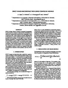
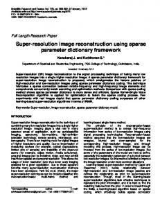
4 Experimental results The proposed algorithm was applied to the ‘castle’ sequence from [17] and the ‘house’ sequence that was captured by a consumer camera (Canon IXUS 400) for testing. For both data sets, the cameras are first calibrated using the factorization-based SFM method [14]. The 3D shape of the surface is then reconstructed using MRF optimization. Fig. 3(a) and Fig. 4(a) show the central images of the two sequences and the sparse points that are reconstructed by SFM. Fig. 4 shows the results of the each major step of the proposed algorithm for the ‘castle’ sequence, and Fig. 3 shows the results for the ‘house’ sequence. Totally 5 consecutive images are selected from the ‘castle’ and 9 images are selected from the ‘house’ for our surface reconstruction. The central image is selected as the reference image. Similar to [10], we first align the world coordinates to the camera coordinates of the central image. Then the depth planes are sampled in the 3D space
(a) Central image with reconstructed points.
(b) Segmentation map.
(c) Tetrahedral mesh for MRF optimization.
(d) Depth map.
Fig. 3. Results for the ‘house’ data set.
with increasing depth to the central camera. The depth difference between two consecutive depth planes was chosen in such a way that every label change results in the pixel displacement of the principal point in the central image by at most 1 pixel in both x and y directions. Fig. 2(b) illustrates the depth planes. A 5 × 5 window was used to compute the intensity variance σ2p of the image patch around pixel p ∈ P . A 17 × 17 window was used to compute the SAD value S p (L) for all depths L ∈ L . The SAD value was computed in R, G, B channels and then averaged. If the projection of the 3D point is outside an image, the SAD value for that image pair is discarded. After we obtain the depths for the centroids of all triangles, depth map is created simply by assigning the depth of the centroid to all pixels within the same triangle. Fig. 3(d) and Fig. 4(h) show the depth maps of the central images for the ‘house’ and ‘castle’ sequences. As we see from the figures, the depths of most pixels are accurately reconstructed. Especially, the depth discontinuities (e.g. the lamp post on the right of Fig. 3(d)) are very well preserved because of the image content adaptive local energies. Due to the use of large triangles as shown in Fig. 3(b) and Fig. 4(g), some small details of the scene are not reconstructed. For applications in which small details are required, the shape obtained by the proposed algorithm can be used as a base shape for further
improvement. For example, by further splitting the triangles, the current 3D shape can be refined to a finer level using the proposed method.
5 Conclusion We have presented an image-based multi-view reconstruction technique for surface reconstruction from multiple images with small or moderate baselines, using MRF optimization. Our principal idea is that the local penalty energy and interaction potential need to be adapted to local image content. This paper proposes techniques to combine various depth cues and prior information to exploit image locality. First, we propose a method to construct a 2D triangular mesh based on the over-segmented image. The generated triangles are well aligned with the object boundaries, and are able to accurately represent the object surface using a minimum number of triangles. Second, we employ various objective and heuristic depth cues do define the penalty and interaction energies, such that the ambiguity among depth labels can be efficiently removed during MRF optimization. Third, based on some simple content analysis methods, we tune both the penalty and interaction energies to the local image content. The experimental results show that the surface of the scene is accurately reconstructed, and the the depth discontinuities are very well preserved because of the content-adaptive local energies. The proposed method is effective for outdoor scene reconstruction.
References 1. Kauffa, P., Atzpadina, N., Fehna, C., Mllera, M., Schreer, O., Smolica, A., Tangera, R.: Depth map creation and image-based rendering for advanced 3dtv services providing interoperability and scalability. Signal Processing: Image Communication 22 (2007) 217–234 2. Zeng, G., Paris, S., Quan, L., Lhuillier, M.: Surface reconstruction by propagating 3d stereo data in multiple 2d images. In: Proc. European Conf. Computer Vision. (2004) 3. Seitz, S.M., Dyer, C.R.: Photorealistic scene reconstruction by voxel coloring. In: Proc. IEEE Conf. Computer Vision and Pattern Recognition. (1997) 1067–1073 4. Paris, S., Sillion, F.X., Quan, L.: A surface reconstruction method using global graph cut optimization. Int. J. Computer Vision 66 (2006) 141–161 5. Vogiatzis, G., Torr, P., Cipolla, R.: Multi-view stereo via volumetric graph-cuts. In: Proc. IEEE Conf. Computer Vision and Pattern Recognition. Volume 2. (2005) 391–398 6. Roy, S., Cox, I.J.: A maximum-flow formulation of the n-camera stereo correspondence problem. In: Proc. Int. Conf. Computer Vision. (1998) 492–499 7. Boykov, Y., Veksler, O., Zabih, R.: Fast approximate energy minimization via graph cuts. IEEE Trans. Pattern Analysis and Machine Intelligence 23 (2003) 1222–1239 8. Sun, J., Zheng, N.N., Shum, H.Y.: Stereo matching using belief propagation. IEEE Trans. Pattern Analysis and Machine Intelligence 25 (2003) 787–800 9. Scharstein, D., Szeliski, R.: A taxonomy and evaluation of dense two-frame stereo correspondence algorithms. Int. J. of Computer Vision 47 (2002) 7–42 10. Kolmogorov, V., Zabih, R.: Multi-camera scene reconstruction via graph cuts. In: Proc. European Conf. Computer Vision. Volume LNCS: 2352. (2002) 82–96 11. : (http://vision.middlebury.edu/MRF/code/ ) 12. et. al., R.S.: A comparative study of energy minimization methods for markov random fields. In: Proc. European Conf. Computer Vision. Volume LNCS 3952. (2006) 16–29 13. : (http://people.cs.uchicago.edu/ ˜ pff/segment/ ) 14. Han, M., Kanade, T.: A perspective factorization method for euclidean reconstruction with uncalibrated cameras. J. Visual. Comput. Animat. (2002) 15. Boykov, Y., Kolmogorov, V.: An experimental comparison of min-cut/max-flow algorithms for energy minimization in vision. IEEE Trans. Pattern Analysis and Machine Intelligence 26 (2004) 1124–1137 16. Felzenszwalb, P.F., Huttenlocher, D.P.: Efficient graph-based image segmentation. Int. J. Computer Vision 59 (2004) 167–181 17. : (http://www.cs.unc.edu/ ˜ marc/ )
(a) Central image with reconstructed points.
(b) Segmentation map.
(c) Segment boundaries.
(d) Triangular mesh by Delaunay triangulation
(e) Splitting of the large triangles.
(f) Final triangular mesh after splitting.
(g) Tetrahedral mesh for MRF optimization.
(h) Depth map.
Fig. 4. Results for the ‘castle’ data set.