Linear Invariant Systems Theory for Signal ...

Linear Invariant Systems Theory for Signal Enhancement A. M. Tom´e , A. R. Teixeira , A. Teixeira, G. Miguel , P. Georgieva , E. W. Lang

Abstract – This paper discusses a linear time invariant (LTI) systems approach to signal enhancement via projective subspace techniques. It provides closed form expressions for the frequency response of data adaptive finite impulse response eigenfilters. An illustrative example using speech enhancement is also presented. Resumo – Este artigo apresenta a aplicac¸a˜ o da teoria de sistemas lineares invariantes no tempo (LTI) na an´alise de t´ecnicas de sub-espac¸o. A resposta em frequˆencia dos filtros resultantes da decomposic¸a˜ o em valores singulares e´ obtida aplicando as propriedades dos sistemas LTI. Keywords – Signal Enhancement, SVD, Subspace-Based Methods

I. I NTRODUCTION Signal enhancement via projective subspace techniques is widely used in speech processing and biomedical signal processing to improve noise-corrupted signals. Different notations or mathematical formalisms are discussed in the literature [1], [2], [3], but singular value decomposition (SVD) is common to all. A data-derived trajectory matrix ˆ From this X is replaced by a low-rank approximation X. ˆ an enhanced version x low-rank matrix X ˆ[k] of the original signal is then obtained employing diagonal averaging [4]. A discussion of these techniques in the frequency domain was given by [5] where it was shown that signal enhancement can be achieved by a bank of finite impulse response filters arranged as parallel pairs of analysis-synthesis filters. The proposed approach was formulated using matrix algebra operations [5], [6], [1].In this work we show that linear invariant system theory provides alternative tools to derive such input-output relations. Analytical expressions for the frequency response of these filters will be given. In addition, the main filter characteristics, i.e. causality and being zero-phase, are deduced. The paper addresses the following three topics: the meaning of SVD in terms of univariate time series analysis; the filter bank interpretation and a few illustrative examples using speech signals. II. U NIVARIATE

TIME - SERIES AND

SVD

Singular value decomposition constitutes the main tool to estimate subspace models for multidimensional data sets. In multi-sensor signal processing, the data vector is naturally formed with samples of different sensors. However, projective subspace techniques can also be applied to univariate time series by forming vectors with sliding windows of the signal. This transformation is called embedding the signal into the space of time-delayed coordinates. Considering a segment of a signal (x[1], x[2], . . . , x[K]), the multidimensional signal is obtained by xk∗ = (x[k], . . . , x[k +

N ]), k = 1, . . . , M = K − N + 1. The lagged vectors lie in a space of dimension N and constitute the rows of the trajectory matrix 

x[1]  x[2]   x[3] X=  . ..  x[M ]

x[2] x[3] x[4] . .. x[M + 1]

... ... ... .. . ...

x[N ] x[N + 1] x[N + 2] . .. x[K]

      

(1)

Note that this matrix has identical entries along its antidiagonals, hence forms an Hankel matrix [1]. There are other alternatives to form the data matrix via embedding the signal in an N − dimensional space which yield a Toeplitz matrix. The latter has identical elements along its diagonals [2]. However, the processing steps are the same, only adapted to cope with the differences in data organization [7]. Following that strategy, the univariate signal is organized into an M × N matrix X whose SVD [8] allows to explain the data set as a product of matrices X = UΣVT , where U and V are orthonormal matrices with dimension M × M and N × N , respectively. The matrix Σ is an M × N matrix with r ≤ min(M, N ) non-zero singular values along the diagonal and zeros everywhere else. The eigenvector matrices (U and V) result from an eigenvalue decomposition of two symmetric and square matrices computed from the data matrix. Assuming that the vectors xk∗ , k = 1, 2 . . . , M , represent the rows of X, the two different square matrices are computed in the following way: • Matrix S = XT X is an N × N matrix where each entry represents the correlations between pairs of entries of the data vectors. It is an outer product matrix corresponding to the non-normalized correlation matrix. If the data is centered, it is also the non-normalized covariance matrix, also called scatter matrix. Its eigenvalue decomposition reads S = VΛVT = VΣT ΣVT . The matrix Λ is a diagonal matrix with at most r ≤ min(M, N ) non-zero eigenvalues corresponding to the square of the singular values. And the eigenvector matrix V is orthonormal, e.g. VT V = I, where I is the identity matrix. • Matrix K = XXT is an M × M matrix where each entry represents the dot product between pairs of vectors of the data set (the rows of X). It is known as kernel matrix or dot product matrix. The eigenvalue decomposition of this matrix reads K = UΛUT = UΣΣT UT . The matrix Λ is a diagonal matrix with at most r ≤

min(M, N ) non-zero eigenvalues and UT U = I is an orthonormal eigenvector matrix. Orthogonal subspace models, like SVD or principal component analysis (PCA), are described solely by the matrix V that defines an orthonormal basis vector matrix of the N − dimensional space of the data [8]. A low-rank approximation of the data matrix X can be expressed as follows ˆ = XVPVT = YPVT X

(2)

where each term means: • matrix Y = XV represents the projection of the data vectors xk∗ ∈ ℜN onto the basis vectors. Each column y∗n represents the projections of all row vectors xk∗ , k = 1, . . . , M onto the n-th basis vector v∗n . • matrix P is a diagonal matrix with diagonal entries equal to 0 ≤ pnn ≤ 1. If pnn = 1, the n − th column of Y is retained, and if pnn = 0, it is replaced by a null vector. In the general case, the scaling factors pnn can be estimated from the eigenvalue spectrum and the related noise variance [1]. ˆ in the original N − • the reconstructed data X dimensional space results from the product with VT ˆ corresponds to a reThus the reconstructed data matrix X duced rank approximation of the original data matrix with a possibly modified eigenvalue spectrum. But the reconstruction does not preserve the Hankel structure of the original data matrix (see eqn. 1). To rectify this, each anti-diagonal element is substituted by the corresponding average of all entries of the anti-diagonal. Finally, the embedding is reversed to obtain the reconstructed signal xˆ[k] which is an enhanced version of the original signal. III. SVD

AS

F ILTER BANKS

Signal enhancement as it was sketched above can also be addressed employing linear invariant systems theory. In the following we discuss the application of a bank of finite impulse response (FIR) filters, where analysis and synthesis filter pairs are connected in parallel. Note that eqn. (2) can be expressed as a weighted superposition of terms related with the non-zero singular values/eigenvalues and corresponding eigenvectors of the subspace model. Employing the subspace model V = [v∗1 , v∗2 , . . . , v∗N ], and using ˆ n are M × N matriblock matrix operations, the terms X ces of rank one. The reconstructed data matrix can then be expressed as ˆ = X =

T T Xv∗1 p11 v∗1 + . . . + Xv∗N pN N v∗N T T y∗1 p11 v∗1 + · · · + y∗N pN N v∗N =

N X

ˆ n(3) X

n=1

where v∗n , n = 1, . . . , N represent analysis or synthesis filter coefficients. In Hansen et al. [5], a filter bank architecture is proposed where formally analysis and synthesis

filters operate on trajectory matrices with a Hankel and a Toeplitz structure, respectively, to include the diagonal averaging [4] during synthesis. However, in the framework of linear invariant systems theory, the filter bank structure needed to achieve the output time series x ˆ[k] should be provided by the input time series x[k] instead of by the trajectory matrix. Hence we propose an approach based on filter responses and related transfer functions rather than on matrix manipulations. As mentioned above, each column y∗n , n = 1, . . . , N of the projected data Y is obtained via y∗n = Xv∗n . Each element of the M × 1 vector y∗n is the dot product between the n−th eigenvector and a row of the data matrix. But this data manipulations can also be formulated as the weighted sum of a sequence of samples of the original time series, yn [k] =

N X i=1

vin x[k + i − 1]

(4)

where 1 ≤ k < M and yn [k] are the elements of the nth column of matrix Y, i.e, y∗n . Therefore, the y∗n has M samples starting by time index k = 1, like in the first column of the matrix X. The entries of the vector v∗n , the n − th column of the subspace model, are the coefficients of an anti-causal finite impulse response (FIR) filter as the output at time index k depends on input samples at time index k, k + 1 . . . k + N − 1. The transfer function Hn (z) of the analysis step can be computed by substituting in eqn. (4) every delay operation by the corresponding z transform [9]. Therefore by P∞ −k transforming x[k] to X(z = x[k]z , x[k ± d] to −∞ ±d z X(z) and yn [k] to Yn (z), the filtering operation can be formulated using the following transfer function

Hn (z) =

Yn (z) = (v1n + v2n z 1 + . . . vN n z (N −1) ) (5) X(z)

This transfer function Hn (z), n = 1, . . . , N results from an output-input ratio and constitutes the analysis block as it decomposes the input into several components yn [k], n = 1, . . . , N . In filter bank terminology, the analysis filter is then followed by the synthesis filter which should combine components to form a new signal. To facilitate the exposition, let’s consider the n-th term of eqn. (3) and assume pnn = 1 for simplicity. In that case the n-th contribution to the reconstructed data matrix is ˆ n = Xv∗n vT = y∗n vT . X ∗n ∗n

(6)

ˆ n is a Therefore each column of the rank-one matrix X scaled version of y∗n 

   ˆ Xn =   

v1n yn [1] v1n yn [2] v1n yn [3] .. .

v2n yn [1] v2n yn [2] v2n yn [3] .. .

... ... ...

vN n yn [1] vN n yn [2] vN n yn [3] .. .

v1n yn [M ] v2n yn [M ] . . . vN n yn [M ]

       (7)

s 1 X x ˆn [k] = vin yn [k − i + 1] Nd

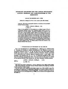
11 7000

10 9

6000

8 frequency−Hz

Obviously, the resulting matrix does not have the Hankel structure of the original matrix X. But by replacing the enˆ n by their average, an Hantries in each anti-diagonal of X kel matrix is obtained again. Interestingly, the diagonal averaging can equally well be formulated as a linear filtering operation (8)

5000

7 6

4000

5 3000

4 3

2000

i=l

2 1000 1

where the quantities Nd , l and s have values according to number of elements in the anti-diagonals of the matrix defined in eqn. (7). More specifically, the response can be sub-divided into a transient and a steady state response according to the following distinction:

0

10

20

30 40 frame number

50

60

11 7000

10 9

6000

• With less than N elements, eqn. (8) represents the transitory response of the filter: – if 1 ≤ k ≤ (N − 1) (upper left corner of the matrix ˆ n ) then we have Nd = k, l = 1 and s = Nd ; X – if (M +1) ≤ k ≤ K (lower right corner of the matrix ˆ n ) then we have Nd = K −k +1, l = N −Nd +1 X and s = N . Note that the entries of the vector v∗n , the n − th column of the subspace model, are the coefficients of a causal finite impulse response (FIR) filter. Both cases can be unified by formally setting ym [k] = 0 for the time indices k < 1 and k > M , and always compute eqn. (8) as in the steady-state case. Therefore, the transfer function for the synthesis filter reads ˆ n (z) X 1 = (v1n +v2n z −1 +. . .+vN n z −(N −1) ) Yn (z) N (9) Notice that the analysis (Hn (z)) and synthesis (Fn (z)) transfer functions differ by a scale factor (1/N ) and by the sign of the powers of z. Therefore the magnitudes of the frequency response of both filters are related by a scale factor (1/N ) and their phases are symmetric. The transfer function of the global system is a cascade formed by the projection step (analysis) and the reconstruction step with diagonal averaging (synthesis) given by

Fn (z) =

Tn (z) =

ˆ n (z) X = Fn (z)Hn (z) = X(z)

N −1 X

tin z i (10)

i=−(N −1)

The coefficients tin result from the product of two polynomials with the same coefficients but powers of z with opposite sign, and then tin = t−in , i = 1, . . . , (N − 1) [9]. Therefore, the frequency response Tn (ejω ) has the following expression

8 frequency−Hz

• With N elements, eqn. (8) represents a steady state response of the filter in the case of N ≤ k ≤ M and we have Nd = N , l = 1 s = N .

5000

7 6

4000

5 3000

4 3

2000

2 1000 1 0

10

20

30 40 frame number

50

60

Fig. 1 - Spectogram of the signal with different SNR:left-SNR=40dB, right-SNR=10dB.

Tn (ejω ) = t0n +

N −1 X

2tin cos(iω)

(11)

i=1

√ where j = −1. The frequency response is a periodic real function, with period equal ω = 2π, hence corresponds to a zero-phase filter. This means that each extracted component x ˆn [k] is always in-phase with its related original x[k]. The orthogonal output sequences yn [k], n = 1 . . . N of the analysis step are filtered versions of the input sequence x[k] and their energy content is given by the eigenvalue associated with the corresponding eigenvector (eigenfilter). The scale factor pnn only changes the amplitude of the sequence yn [k]. The total transfer function is finally obtained by adding the transfer functions of the parallel branches of the filter bank. The resulting output x ˆ[k] is a sum of the selected signals x ˆn [k], e.g, the outputs of the cascaded filter pairs formed by Hn (z) and Fn (z). Notice, that the embedding of the time-series as suggested by (1) leads to an anticausal filter for the analysis step and to a causal filter for the synthesis step. Using alternative embedding procedures, this property of the filters can interchange. Though examples of frequency responses of the eigenfilters are shown graphically in [5], no analytical expressions of the filter responses are given. Instead, the present work also deduces such closed-form analytical expressions for the analysis and synthesis filters. Note that frequency responses of the component filters Hn (z) and Fn (z) cannot be given in closedform similar to Tn (z) in (11) due to lacking symmetry properties of their coefficients [9]. But notice that the absolute values of the frequency responses of all the filters have the

0.9

7000

7000

0.7

6000

0.6

5000

0.5

4000

0.4

3000

0.3

2000

0.2

1000

0.1

0.8 6000 5000

0.6

4000

0.5 0.4

3000

frequency− Hz

frequency−Hz

0.7

0.3 2000 0.2 1000 0

0.1 10

20

30 40 frame number

50

60

0

0

5

10

15 20 filter number

25

30

0.8

0.9

7000

7000

0.7

0.8 6000

0.7

5000

0.6

4000

0.5 0.4

3000

0.6 frequency− Hz

frequency−Hz

6000

0.3 2000

5000 0.5 4000 0.4 3000

0.3

2000

0.2

1000

0.1

0.2 1000 0

0.1 10

20

30 40 frame number

50

60

0

0

5

10

15 20 filter number

25

30

0.8

7000

0.6

7000

0.5

6000

0.7

5000 0.4 4000 0.3 3000 0.2

2000

0.1

1000 0

10

20

30 40 frame number

50

60

0

Fig. 2 - Frequency responses of T1 (z), related with largest eigenvalue, along the frames computing model with :top-SNR=40dB, middleSNR=10dB , bottom-SNR=0dB

same profile. IV. D ISCUSSION

AND

C ONCLUSION

In this section we present illustrative examples of the frequency response of eigenfilters for a segment of a speech signal corrupted by additive gaussian noise. Fig. 1 shows the frequency content of a noisy speech signal in each frame (spectrogram). Each frame correspond to a segment of 25ms (400 samples) with 60% of overlap between the frames. In the first spectrogram the energy of the signal is concentrated in the frames 15 − 45 corresponding to frequencies f < 2000Hz. With decreasing the SNR, the speech signal becomes increasingly corrupted and the frequency content is distributed more uniformly (see Fig. 1, right). The orthogonal subspace model V was computed for each frame using K = 400 samples and an embedding dimension N = 30. Fig 2 shows the frequency response of T1 (z), i.e. of

0.6 frequency− Hz

frequency− Hz

6000

5000 0.5 4000

0.4

3000

0.3

2000

0.2

1000

0.1

0

5

10

15 20 filter number

25

30

Fig. 3 - Frequency responses of Tn (z), n = 1, . . . , N for 30th frame using:top-SNR=40dB, middle-SNR=10dB , bottom-SNR=0dB

the analysis/synthesis filter that corresponds to the largest eigenvalue of the subspace models. This filter is clearly centered in the region of the highest energy of the input signals. If the SNR is high (figure on left), the passband of the filter matches the signal. Even when the energy of the signal is low, the filter has its passband in low frequency range. When the noise level increases, the passband of the filter moves towards the high frequency range for the frames without signal information (see figure on middle). But when SN R = 0dB, the filter is always centered on the high-frequency range both in frames without or with active voice signals. Fig. 3 shows the frequency response of Tn (z), n = 1 . . . 30 computed using a frame with active voice (the 30th frame). The differences on the profile of the frequency responses is obvious. The filters were ordered according the values of the eigenvalues. It can be seen that when the SNR is high, the first filters, associated with the largest eigenvalues, have their passband centered in the low frequency range, and the last filters, as-

sociated with the smallest eigenvalues, are centered in the high-frequency range. Decreasing the SNR, the filters associated with the highest eigenvalues have passbands both in the low-frequency band and in the high-frequency band (see figure on middle). However, for SN R = 10dB, the first five filters still concentrate their passband in low frequency range. Finally, when SN R = 0dB, the filters with their passband in the high frequency range are the ones corresponding to the largest eigenvalues, while the filters centered in low frequency range correspond to the smallest eigenvalues. The interpretation of subspace-based methods as filter banks helps to attain a clear-cut insight into the outcomes of the method. By applying a linear invariant system theory approach, analytical expressions of the frequency response are deduced in this work. These results thus corroborate the properties of the SVD steps referred to in previous works [5], [4], [6]. By the frequency responses of the filter bank, corresponding to the basis vectors of the subspace model, the frequency content of the different components can be attained easily. Eigenfilters are data adaptive, and the relevance of one component to the energy of the input signal is deduced from the corresponding eigenvalue. Moreover, the frequency profile of each component is determined only at the projection step. However, in order to get a component in phase with the input signal, the diagonal averaging is required. R EFERENCES [1] Per Christian Hansen and S. Holdt Jensen, “Subspace-based noise reduction for speech signals via diagonal and triangular matrix decompositions: Survey and analysis”, Eurasip Journal on Advances in Signal Processing, vol. Vol 2007, 2007. [2] Nina Golyandina, Vladimir Nekrutkin, and Anatoly Zhigljavsky, Analysis of Time Series Structure: SSA and Related Techniques, Chapman & HALL/CRC, 2001. [3] M. Ghil, M.R. Allen, M. D. Dettinger, and K. Ide, “Advanced spectral methods for climatic time series”, Reviews of Geophysics, vol. 40, no. 1, pp. 3.1–3.41, 2002. [4] I. Dologlou and G. Carayannis, “Physical interpretation of signal reconstruction from reduced rank matrices”, IEEE Transactions on Signal Processing, vol. 39, no. 7, pp. 1681–1682, 1991. [5] Per Christian Hansen and Soren Holdt Jensen, “FIR filter representations of reduced-rank noise reduction”, IEEE Transactions on Signal Processing, vol. 46, no. 6, pp. 1737–1741, 1998. [6] Kris Hermus, Patrick Wambacq, and Hugo Van hamme, “A review of signal subspace speech enhancement and its application to noise robust speech recognition”, Eurasip Journal on Advances in Signal Processing, 2007. [7] A. R. Teixeira, A. M. Tom´e, M. B¨ohm, C. G. Puntonet, and E. W. Lang, “How to apply non-linear subspace techniques to univariate biomedical time series”, IEEE Transactions on Instrumentation & Measurement, vol. 58, no. 8, pp. 2433–2443, 2009. [8] K. I. Diamantaras and S.Y. Kung, Principal Component Neural Networks, Theory and Applications, Wiley, 1996. [9] Leland B. Jackson, Digital Filters and Signal Processing, Kluwer Academic Publishers, 1996.