On Switched Control Design of Linear Time-Invariant Systems with ...

Hindawi Publishing Corporation Mathematical Problems in Engineering Volume 2013, Article ID 595029, 10 pages http://dx.doi.org/10.1155/2013/595029

Research Article On Switched Control Design of Linear Time-Invariant Systems with Polytopic Uncertainties Wallysonn A. de Souza,1 Marcelo C. M. Teixeira,2 Máira P. A. Santim,3 Rodrigo Cardim,2 and Edvaldo Assunção2 1

Department of Academic Areas of Jata´ı, Federal Institute of Education, Science and Technology of Goiás (IFG), Campus Jata´ı, 75804-020 Jata´ı, GO, Brazil 2 Department of Electrical Engineering, UNESP, Univ Estadual Paulista, Campus de Ilha Solteira, 15385-000 Ilha Solteira, SP, Brazil 3 Department of Computer, Telecommunication, Control, and Automation Engineering, Faculdade of Science and Technology of Montes Claros (FACIT), Campus II, 39400-141 Montes Claros, MG, Brazil Correspondence should be addressed to Wallysonn A. de Souza; [email protected] Received 17 January 2013; Accepted 12 April 2013 Academic Editor: Oleg V. Gendelman Copyright © 2013 Wallysonn A. de Souza et al. This is an open access article distributed under the Creative Commons Attribution License, which permits unrestricted use, distribution, and reproduction in any medium, provided the original work is properly cited. This paper proposes a new switched control design method for some classes of linear time-invariant systems with polytopic uncertainties. This method uses a quadratic Lyapunov function to design the feedback controller gains based on linear matrix inequalities (LMIs). The controller gain is chosen by a switching law that returns the smallest value of the time derivative of the Lyapunov function. The proposed methodology offers less conservative alternative than the well-known controller for uncertain systems with only one state feedback gain. The control design of a magnetic levitator illustrates the procedure.

1. Introduction In recent years, there has been much interest in studying switched systems, due to the considerable advance in this research field, initiating mainly with [1–4]. For linear timeinvariant systems, the transient response can be improved through switching controllers [5], as can be seen, for instance, in [6–9]. In general, most papers in the area of switched linear systems utilize multiple Lyapunov functions [10–14]. A design method that is applicable to a large class of switched controllers for linear systems with input signals, formulated with bilinear matrix inequalities (BMIs), is proposed in [10]. The switching law defines regions where different subsystems are activated, resulting in a switched linear system that is exponentially stable. Study results on the stability analysis and stabilization of switched systems can be seen in [11], which presents necessary and sufficient conditions for asymptotic stability. Moreover, the problem of switching stabilizability is studied, investigating under what conditions it is possible

to stabilize a switched system by designing switching control laws. Necessary and sufficient conditions for switched linear systems with polytopic uncertainties to be quadratically stabilizable via state feedback can be found in [13]. The design of the robust state feedback control for continuous-time systems subject to norm bounded uncertainty can be seen in [12], where the switching rule, as well as the state feedback gains, is determined from the minimization of a guaranteed cost function derived from a multiobjective criterion. The paper [14] presents a generalization of the results proposed in [12] and offers a procedure that finds, simultaneously, a set of state feedback gains and a switching rule to orchestrate them, rendering the equilibrium point of closed-loop system globally asymptotically stable for all time-varying uncertain parameters under consideration and assuring a guaranteed H2 cost. Although outnumbered, there are papers about switched linear systems using a common Lyapunov function as in [15, 16]. In [15], the stability of switched linear systems with polytopic uncertainties was studied. Some criteria for globally

2

Mathematical Problems in Engineering

exponential stability were also established, in which all the vertex matrices of the switched systems are commutative pairwise, thus generalizing the existing results for switched linear systems without uncertainty. In [16] the quadratic stability for continuous-time and discrete-time switched linear systems with a switching rule using a single symmetric positive definite matrix, which depends on system states vector, was studied. This paper proposes a new methodology for switched control design of a class of linear systems with polytopic uncertainties. This method uses a common Lyapunov function and quadratic stability for designing the state feedback controller gains based on linear matrix inequalities (LMIs). The proposed controller chooses a gain from a set of gains by means of a suitable switching law that returns the smallest value of the Lyapunov function time derivative. The proposed methodology allows a less conservative LMI-based design than the traditional method for uncertain plants that considers only one state feedback controller gain [17]. To confirm the advantages of the proposed methodology, figures comparing the regions of feasibility of the proposed methodology with the one state feedback gain classical method are presented. To compare the performance of the proposed control law with the classical control law, an application in the magnetic levitator control was simulated. The computational implementations were carried out using the modelling language YALMIP [18] with the solver SeDuMi [19]. For convenience, in some places, the following notation is used: K𝑟 = {1, 2, . . . , 𝑟} , 𝑉 (𝑥 (𝑡)) = 𝑉,

𝑥 (𝑡) = 𝑥, ‖𝑥‖2 = √𝑥𝑇𝑥,

𝑟

(𝐴, 𝐵, 𝐾) (𝛼) = ∑𝛼𝑖 (𝐴 𝑖 , 𝐵𝑖 , 𝐾𝑖 ) , 𝑖=1 𝑟

∑𝛼𝑖 = 1, 𝑖=1

(1)

with 𝛼𝑖 ≥ 0, (2) 𝑇

𝛼 = [𝛼1 , 𝛼2 , . . . , 𝛼𝑟 ] ,

where 𝐾 ∈ R𝑚×𝑛 . Replacing (4) in (3), one obtains the feedback system 𝑟

𝑥̇ (𝑡) = 𝐴 (𝛼) 𝑥 (𝑡) − 𝐵 (𝛼) 𝐾𝑥 (𝑡) = ∑𝛼𝑖 (𝐴 𝑖 − 𝐵𝑖 𝐾) 𝑥 (𝑡) . 𝑖=1

(5) Define a feedback control law with the state vector as 𝑟

𝑢 (𝑡) = 𝑢𝛼 (𝑡) = −∑𝛼𝑖 𝐾𝑖 𝑥 (𝑡) = −𝐾 (𝛼) 𝑥 (𝑡) ,

where 𝐾𝑖 ∈ R𝑚×𝑛 , 𝑖 ∈ K𝑟 . Considering (2) and from (6) and (3), 𝑥̇ (𝑡) = 𝐴 (𝛼) 𝑥 (𝑡) − 𝐵 (𝛼) 𝐾 (𝛼) 𝑥 (𝑡) 𝑟

𝑟

= ∑ ∑𝛼𝑖 𝛼𝑗 (𝐴 𝑖 − 𝐵𝑖 𝐾𝑗 ) 𝑥 (𝑡) . 𝑖=1 𝑗=1

2.1. Stability of Linear Systems via LMIs. This section presents some results on stability and control of linear systems with polytopic uncertainties. Theorem 1 (see [20]). The linear system with polytopic uncertainties given in (5) is quadratically stabilizable if and only if there exist a common symmetric positive definite matrix 𝑋 and 𝑀 ∈ R𝑚×𝑛 such that, for all 𝑖 ∈ K𝑟 , 𝑋𝐴𝑇𝑖 + 𝐴 𝑖 𝑋 − 𝐵𝑖 𝑀 − 𝑀𝑇 𝐵𝑖𝑇 ≺ 0.

(8)

If there exists such a solution, the controller gain is given by 𝐾 = 𝑀𝑋−1 . Theorem 2. The equilibrium point 𝑥 = 0 of the linear system with polytopic uncertainties given in (7) is asymptotically stable in the large if there exist a common symmetric positive definite matrix 𝑋 and 𝑀𝑖 ∈ R𝑚×𝑛 such that, for all 𝑖, 𝑗 ∈ K𝑟 , the following LMIs hold:

𝑇

(𝐴 𝑖 + 𝐴 𝑗 ) 𝑋 + 𝑋(𝐴 𝑖 + 𝐴 𝑗 ) − 𝐵𝑖 𝑀𝑗 − 𝐵𝑗 𝑀𝑖 − 𝑀𝑖𝑇 𝐵𝑗𝑇 − 𝑀𝑗𝑇 𝐵𝑖𝑇 ⪯ 0,

2. Linear Systems with Polytopic Uncertainties Consider the linear system with polytopic uncertainties (3)

where 𝑥(𝑡) ∈ R𝑛 is the state vector, 𝑢(𝑡) ∈ R𝑚 is the control input, 𝐴(𝛼) and 𝐵(𝛼) as in (2), with 𝐴 𝑖 ∈ R𝑛×𝑛 and 𝐵𝑖 ∈ R𝑛×𝑚 for 𝑖 ∈ K𝑟 . Assuming that all state variables are available for feedback, the control law largely used in the literature is given by [17]: 𝑢 (𝑡) = −𝐾𝑥 (𝑡) ,

(7)

𝑋𝐴𝑇𝑖 + 𝐴 𝑖 𝑋 − 𝐵𝑖 𝑀𝑖 − 𝑀𝑖𝑇 𝐵𝑖𝑇 ≺ 0,

where 𝑟 = 2𝑠 and 𝑠 is the number of uncertain parameters in the plant.

𝑥̇ (𝑡) = 𝐴 (𝛼) 𝑥 (𝑡) + 𝐵 (𝛼) 𝑢 (𝑡) ,

(6)

𝑖=1

(4)

(9)

𝑖 < 𝑗.

If (9) are feasible, the controller gains are given by 𝐾𝑖 = 𝑀𝑖 𝑋−1 , 𝑖 ∈ K𝑟 . Proof. Consider a quadratic Lyapunov candidate function 𝑉 = 𝑥𝑇 𝑃𝑥. Thus, from (7) note that 𝑉̇ = 𝑥̇𝑇 𝑃𝑥 + 𝑥𝑇 𝑃𝑥̇ 𝑟

𝑟

𝑇

= ∑ ∑𝛼𝑖 𝛼𝑗 𝑥𝑇 (𝐴 𝑖 − 𝐵𝑖 𝐾𝑗 ) 𝑃𝑥 𝑖=1 𝑗=1

𝑟

𝑟

+ 𝑥𝑇 𝑃∑ ∑ 𝛼𝑖 𝛼𝑗 (𝐴 𝑖 − 𝐵𝑖 𝐾𝑗 ) 𝑥 𝑖=1 𝑗=1


3

𝑟

positive definite matrix 𝑋 and 𝑀 ∈ R𝑚×𝑛 such that, for all 𝑖 ∈ K𝑟 , the following LMIs are satisfied:

= 𝑥𝑇 [∑𝛼𝑖2 (𝐴𝑇𝑖 𝑃 + 𝑃𝐴 𝑖 − 𝐾𝑖𝑇 𝐵𝑖𝑇 𝑃 − 𝑃𝐵𝑖 𝐾𝑖 )] 𝑥 𝑖=1

+𝑥

𝑇[

𝑟−1

𝑟

∑ ∑

[ 𝑖=1 𝑗=1+𝑖

𝛼𝑖 𝛼𝑗 (𝐴𝑇𝑖 𝑃

+ 𝑃𝐴 𝑖 +

𝐴𝑇𝑗 𝑃

𝑋𝐴𝑇𝑖 + 𝐴 𝑖 𝑋 − 𝐵𝑖 𝑀 − 𝑀𝑇 𝐵𝑖𝑇 + 2𝛽𝑋 ≺ 0.

+ 𝑃𝐴 𝑗

If there exists such a solution, the controller gain is given by 𝐾 = 𝑀𝑋−1 .

− 𝐾𝑗𝑇𝐵𝑖𝑇 𝑃 − 𝑃𝐵𝑖 𝐾𝑗

Proof. It is similar to that of Theorem 1, considering 𝑉̇ ≤ −2𝛽𝑉 [17].

−𝐾𝑖𝑇 𝐵𝑗𝑇 𝑃 − 𝑃𝐵𝑗 𝐾𝑖 )] 𝑥. ] (10) Now, 𝛼𝑖 ≥ 0, 𝑖 ∈ K𝑟 and ∑𝑟𝑖=1 𝛼𝑖 = 1. Then, from (10), 𝑉̇ < 0 (for 𝑥 ≠ 0) if for 𝑖, 𝑗 ∈ K𝑟 𝐴𝑇𝑖 𝑃 + 𝑃𝐴 𝑖 − 𝐾𝑖𝑇 𝐵𝑖𝑇 𝑃 − 𝑃𝐵𝑖 𝐾𝑖 ≺ 0, 𝐴𝑇𝑖 𝑃

+ 𝑃𝐴 𝑖 +

𝐴𝑇𝑗 𝑃

+ 𝑃𝐴 𝑗 −

𝐾𝑗𝑇 𝐵𝑖𝑇 𝑃

− 𝐾𝑖𝑇 𝐵𝑗𝑇 𝑃 − 𝑃𝐵𝑗 𝐾𝑖 ⪯ 0,

− 𝑃𝐵𝑖 𝐾𝑗

(11)

(𝐴 𝑖 + 𝐴 𝑗 ) 𝑋 + 𝑋(𝐴 𝑖 + 𝐴 𝑗 ) − 𝐵𝑖 𝑀𝑗 − 𝐵𝑗 𝑀𝑖 − 𝑀𝑖𝑇 𝐵𝑗𝑇 − 𝑀𝑗𝑇 𝐵𝑖𝑇 + 4𝛽𝑋 ⪯ 0,

𝑖 < 𝑗. (15)

Corollary 3. If 𝐵1 = 𝐵2 = ⋅ ⋅ ⋅ = 𝐵𝑟 = 𝐵, then the equilibrium point 𝑥 = 0 of the linear system with polytopic uncertainties given in (7) is asymptotically stable in the large if there exist a symmetric positive definite matrix 𝑋 and 𝑀𝑖 ∈ R𝑚×𝑛 , such that for all 𝑖 ∈ K𝑟 , (12)

If (12) is feasible, the controller gains are given by 𝐾𝑖 = 𝑀𝑖 𝑋−1 , 𝑖 ∈ K𝑟 . Proof. It is similar to the proof of Theorem 2, considering 𝐵𝑖 = ̇ = 𝐵, 𝑖 ∈ K𝑟 , and noting that now (7) can be rewritten as 𝑥(𝑡) ∑𝑟𝑖=1 𝛼𝑖 (𝐴 𝑖 − 𝐵𝐾𝑖 )𝑥(𝑡). In a control design, it is important to assure stability and usually other indices of performance for the controlled system, such as the setting time, constraints on input control and output signals. The setting time is related to the decay rate of the system (5), (or the largest Lyapunov exponent) which is defined as the largest 𝛽 > 0 such that 𝑡→∞

𝑋𝐴𝑇𝑖 + 𝐴 𝑖 𝑋 − 𝐵𝑖 𝑀𝑖 − 𝑀𝑖𝑇 𝐵𝑖𝑇 + 2𝛽𝑋 ≺ 0, 𝑇

Defining 𝑋 = 𝑃−1 , 𝑀𝑖 = 𝐾𝑖 𝑋 and pre- and postmultiplying (11) by 𝑋, one obtains (9). The proof is concluded.

lim 𝑒𝛽𝑡 ‖𝑥 (𝑡)‖2 = 0

Theorem 5. The equilibrium point 𝑥 = 0 of the linear system with polytopic uncertainties given in (7) is asymptotically stable in the large, with decay rate greater than or equal to 𝛽, if there exist a common symmetric positive definite matrix 𝑋 and 𝑀𝑖 ∈ R𝑚×𝑛 such that, for all 𝑖, 𝑗 ∈ K𝑟 ,

𝑖 < 𝑗.

𝑋𝐴𝑇𝑖 + 𝐴 𝑖 𝑋 − 𝐵𝑀𝑖 − 𝑀𝑖𝑇 𝐵𝑇 ≺ 0.

(14)

(13)

holds for all trajectories 𝑥(𝑡). As in [17, page 66], one can use a quadratic Lyapunov function 𝑉 = 𝑥𝑇 𝑃𝑥 to establish a lower bound 𝛽 for the decay rate, considering the condition 𝑉̇ ≤ −2𝛽𝑉 for all trajectories 𝑥. Theorem 4 (see [17]). The linear system with polytopic uncertainties given in (5) is quadratically stabilizable, with decay rate greater than or equal to 𝛽, if and only if there exist a symmetric

If (15) are feasible, the gains are given by 𝐾𝑖 = 𝑀𝑖 𝑋−1 , 𝑖 ∈ K𝑟 . Proof. The proof is similar to that of Theorem 2, considering 𝑉̇ ≤ −2𝛽𝑉. One can constraint the norm of the controller gains by imposing restrictions on 𝑀𝑖 , 𝑖 ∈ K𝑟 , and 𝑋−1 as in [21]. Thus, given the constants 𝜂 > 0 and 𝜂𝑥 > 0, imposing that 𝑀𝑖𝑇 𝑀𝑖 ≺ 𝜂𝐼𝑛 , 𝑖 ∈ K𝑟 , and 𝑋−1 ≺ 𝜂𝑥 𝐼𝑛 , then a constraint on the controller gains may be established by the following theorem [21]. Theorem 6 (see [21]). The constraint on the norm of the controller gains such that 𝐾𝑖 𝐾𝑖𝑇 ≤ 𝜂𝜂𝑥2 𝐼𝑚 , 𝑖 ∈ K𝑟 is enforced if there exist constants 𝜂 > 0 and 𝜂𝑥 > 0, such that the LMIs from Theorems 2 or 5 (or 1 or 4 replacing 𝐾𝑖 = 𝐾 and also 𝑀𝑖 = 𝑀), with the LMIs below hold: [

𝜂𝑥 𝐼𝑛 𝐼𝑛 ] ⪰ 0, 𝐼𝑛 𝑋

[

𝜂𝐼𝑛 𝑀𝑖𝑇 ] ⪰ 0, 𝑀𝑖 𝐼𝑚

𝑖 ∈ K𝑟 .

(16)

Proof. The proof is similar to that presented in [21].

3. Case 1: Linear Systems with a Constant Matrix 𝐵(𝛼) = 𝐵 In this section, the design of a switched controller for the uncertain system (3) is proposed, assuming that 𝐵(𝛼) = 𝐵 is a constant matrix, now given by 𝑥̇ (𝑡) = 𝐴 (𝛼) 𝑥 (𝑡) + 𝐵𝑢 (𝑡) .

(17)

Suppose that (12) is feasible for all 𝑖 ∈ K𝑟 , and let 𝐾𝑖 = 𝑀𝑖 𝑋−1 , 𝑖 ∈ K𝑟 , the gains of the controller given in (6), and

4


𝑃 = 𝑋−1 obtained from the conditions of Corollary 3. Then, define the switched controller 𝑢 (𝑡) = 𝑢𝜎 (𝑡) = −𝐾𝜎 𝑥 (𝑡) , 𝜎 = arg min {−𝑥(𝑡)𝑇 𝑃𝐵𝐾𝑖 𝑥 (𝑡)} ,

𝜎 ∈ K𝑟 .

𝑖∈K𝑟

(18)

Note that, in (18) for a given 𝑡, the switching law 𝜎 can be obtained by calculating −𝑥(𝑡)𝑇 𝑃𝐵𝐾𝑖 𝑥(𝑡), for 𝑖 ∈ K𝑟 , and then considering the index set Ω(𝑡) = {𝑗 ∈ K𝑟 : −𝑥(𝑡)𝑇 𝑃𝐵𝐾𝑗 𝑥(𝑡) ≤ −𝑥(𝑡)𝑇 𝑃𝐵𝐾𝑖 𝑥(𝑡), ∀𝑖 ∈ K𝑟 }. The switching index 𝜎 can be given by 𝜎(𝑡) = 𝑗 ∈ Ω such that 𝑗 ≤ 𝑖, for all 𝑖 ∈ Ω(𝑡). The implementation of (18) in a control application can be done using analog and/or digital electronics. Further details on this subject can be found, for instance, in [22, 23]. Therefore, from (2), the controlled system (17) and (18) is given by 𝑟

and therefore 𝑉𝑢̇ 𝜎 (𝑥(𝑡)) < 0 for 𝑥(𝑡) ≠ 0, ensuring that the equilibrium point 𝑥 = 0 of the controlled system (17) and (18) is asymptotically stable in the large. Thus, Corollary 3 can be used to project the gains 𝐾1 , 𝐾2 , . . . , 𝐾𝑟 and the matrix 𝑃 = 𝑋−1 of the switched control law (18). Additionally, note that the switched control law (18) does not use the uncertain variables 𝛼𝑖 , 𝑖 ∈ K𝑟 , which would be necessary to implement the control law (6). Furthermore, it also offers an alternative less conservative than the well-known control law for uncertain systems presented in (4), with only one controller gain 𝐾.

4. Case 2: Linear System with an Uncertain Matrix 𝐵(𝛼) In this case, the linear system with polytopic uncertainties will be considered as given in (3); with 𝛼𝑖 , 𝑖 ∈ K𝑟 , defined in (2), namely,

𝑥̇ (𝑡) = 𝐴 (𝛼) 𝑥 (𝑡) + 𝐵𝑢𝜎 (𝑡) = ∑𝛼𝑖 (𝐴 𝑖 − 𝐵𝐾𝜎 ) 𝑥 (𝑡) . (19)

̂ (𝛼) 𝑥̂ (𝑡) + 𝐵̂ (𝛼) 𝑢 (𝑡) , ̂̇ (𝑡) = 𝐴 𝑥

𝑖=1

Theorem 7. Assume that the conditions of Corollary 3, related to the system (17) with the control law (6), hold and obtain 𝐾𝑖 = 𝑀𝑖 𝑋−1 , 𝑖 ∈ K𝑟 , and 𝑃 = 𝑋−1 . Then, the switched control law (18) makes the equilibrium point 𝑥 = 0, of the system (17), asymptotically stable in the large. Proof. Consider a quadratic Lyapunov candidate function 𝑉 = 𝑥𝑇 𝑃𝑥. Define 𝑉𝑢̇ 𝛼 and 𝑉𝑢̇ 𝜎 , the derivatives of 𝑉 for the system (17), with the control laws (6) and (18), respectively. Then, from (17) and (18), 𝑉𝑢̇ 𝜎 = 2𝑥 𝑃𝑥̇ = 2𝑥 𝑃 (𝐴 (𝛼) 𝑥 + 𝐵𝑢𝜎 ) 𝑇

𝑟

̂𝑖 , ̂ (𝛼) = ∑𝛼𝑖 𝐴 𝐴 𝑖=1

̇ (𝑡) = V1 (𝑡) , 𝑥𝑛+1

̇ 𝑥𝑛+𝑚 (𝑡) = V𝑚 (𝑡) , or equivalently as presented in [24], (25)

where

and from (20), the switching law given in (18) and (6), observe that 𝑉𝑢̇ 𝜎 = 2𝑥𝑇 𝑃𝐴 (𝛼) 𝑥 + 2min {𝑥𝑇 𝑃𝐵 (−𝐾𝑖 ) 𝑥}

𝑇

𝑥 = [𝑥̂𝑇 𝑥𝑛+1 ⋅ ⋅ ⋅ 𝑥𝑛+𝑚 ] , 𝐴 (𝛼) = [

𝑖∈K𝑟

𝑟

𝑖=1

𝑥̇ (𝑡) = 𝐴 (𝛼) 𝑥 (𝑡) + 𝐵V (𝑡) ,

(21)

𝑖=1

≤ 2𝑥𝑇 𝑃𝐴 (𝛼) 𝑥 + 2𝑥𝑇 𝑃𝐵 (−∑𝛼𝑖 𝐾𝑖 ) 𝑥

(24)

.. .

𝑟

𝑖∈K𝑟

𝑖=1

̂ (𝛼) 𝑥̂ (𝑡) + 𝐵̂ (𝛼) 𝑢 (𝑡) , ̂̇ (𝑡) = 𝐴 𝑥

(20)

From (2), ∑𝑟𝑖=1 𝛼𝑖 = 1 and 𝛼𝑖 ≥ 0, 𝑖 ∈ K𝑟 . Thus, note that min {𝑥𝑇 𝑃𝐵 (−𝐾𝑖 ) 𝑥} ≤ 𝑥𝑇 𝑃𝐵 (−∑𝛼𝑖 𝐾𝑖 ) 𝑥,

(23)

Let V(𝑡) ∈ R𝑚 be the time derivative of the control input ̇ (𝑡) = vector 𝑢(𝑡) ∈ R𝑚 . Define 𝑥𝑛+𝑙 (𝑡) and V𝑙 (𝑡), such that 𝑥𝑛+𝑙 𝑢̇𝑙 (𝑡) = V𝑙 (𝑡), 𝑙 = 1, 2, . . . , 𝑚. Thus, one obtains the following system:

𝑇

= 2𝑥𝑇 𝑃𝐴 (𝛼) 𝑥 + 2𝑥𝑇 𝑃𝐵 (−𝐾𝜎 ) 𝑥.

𝑟

𝐵̂ (𝛼) = ∑𝛼𝑖 𝐵̂𝑖 .

(22)

= 2𝑥𝑇 𝑃 (𝐴 (𝛼) − 𝐵𝐾 (𝛼)) 𝑥 = 2𝑥𝑇 𝑃 (𝐴 (𝛼) 𝑥 + 𝐵𝑢𝛼 ) = 𝑉𝑢̇ 𝛼 .

̂ (𝛼) 𝐵̂ (𝛼) 𝐴 ], 0𝑚×𝑛 0𝑚×𝑚

𝐵=[

0𝑛×𝑚 ]. 𝐼𝑚×𝑚

(26)

After the considerations above, note that the system (25) is similar to the system (17), and therefore the control problem falls into Case 1. Thus, one can adopt the procedure stated in Case 1 for designing a switched control law V(𝑡) = −𝐾𝜎 𝑥(𝑡), 𝐾𝜎 ∈ R𝑛+𝑚 .

Therefore, 𝑉𝑢̇ 𝜎 (𝑥(𝑡)) ≤ 𝑉𝑢̇ 𝛼 (𝑥(𝑡)) and the proof is concluded.

5. Case 3: Linear System with Uncertainty in the Control Signal

Remark 8. Theorem 7 shows that if the conditions of Corollary 3 are satisfied, then 𝑉𝑢̇ 𝛼 (𝑥(𝑡)) < 0 for all 𝑥(𝑡) ≠ 0

In this case, it is assumed that the system (3) is the result of a linearization process of a plant 𝑥̇ = 𝑓(𝑥, 𝑢), at an equilibrium


5

point 𝑥 = 𝑥0 and the respective control input 𝑢 = 𝑢0 . Suppose that 𝑥0 is known, 𝑢0 is uncertain because it depends on the plant uncertainties, but 0 < 𝑢0 ∈ [𝑢0min , 𝑢0max ] where 𝑢0min and 𝑢0max are known, and the linearized system is given by (2) and 𝑥̇ (𝑡) = 𝐴 (𝛼) 𝑥 (𝑡) + 𝐵 (𝛼) 𝑢 (𝑡) ,

for the system (27), with the control laws (6) and (30), (31), respectively. Then, 𝑉𝑢̇ (𝜎,𝜉) = 2𝑥𝑇 𝑃𝑥̇ = 2𝑥𝑇 𝑃 (𝐴 (𝛼) 𝑥 + 𝐵𝑔 (𝛼) 𝑢(𝜎,𝜉) ) = 2𝑥𝑇 𝑃 [𝐴 (𝛼) 𝑥 − 𝐵 (𝛼) 𝐾 (𝛼) 𝑥 + 𝐵𝑔 (𝛼)

(27)

where 𝑥(𝑡) = 𝑥(𝑡) − 𝑥0 , 𝑥(𝑡) is the state vector of the plant; 𝑢(𝑡) = 𝑢(𝑡) − 𝑢0 , 𝑢(𝑡) is the control signal of the plant. Now suppose that 𝐵(𝛼) can be written as follows: 𝐵 (𝛼) = 𝐵𝑔 (𝛼) ,

(28)

where 𝐵 is a constant matrix and 𝑔(𝛼) > 0, for all 𝛼 given in (2), is an bounded function that depends on uncertain parameters 𝛼. Thus, the system (27) can be written as follows:

× (𝑢(𝜎,𝜉) − 𝑢0 + 𝐾 (𝛼) 𝑥)] = 𝑉𝑢̇ 𝛼 + 2𝑥𝑇 𝑃𝐵𝑔 (𝛼) (−𝐾𝜎 𝑥 + 𝛾𝜉 − 𝑢0 + 𝐾 (𝛼) 𝑥)

(32)

= 𝑉𝑢̇ 𝛼 + 2𝑔 (𝛼) min {−𝑥𝑇𝑃𝐵𝐾𝑖 𝑥} 𝑖∈K𝑟

+ 2𝑔 (𝛼) 𝑥𝑇 𝑃𝐵 [𝛾𝜉 − 𝑢0 + 𝐾 (𝛼) 𝑥] . Remembering that 𝛼𝑖 ≥ 0, 𝑖 ∈ K𝑟 and ∑𝑟𝑖=1 𝛼𝑖 = 1, 𝑔(𝛼) > 0, 𝑔(𝛼)𝐵 = 𝐵(𝛼) and noting that min𝑖∈K𝑟 {−𝑥𝑇𝑃𝐵𝐾𝑖 𝑥} ≤ −𝑥𝑇 𝑃𝐵(∑𝑟𝑖=1 𝛼𝑖 𝐾𝑖 )𝑥, from (32) 𝑟

𝑥̇ (𝑡) = 𝐴 (𝛼) 𝑥 (𝑡) + 𝐵 (𝛼) 𝑢 (𝑡) = 𝐴 (𝛼) 𝑥 (𝑡) + 𝐵𝑔 (𝛼) 𝑢 (𝑡) . (29) Assume that the gains 𝐾𝑖 = 𝑀𝑖 𝑋−1 , 𝑖 ∈ K𝑟 , and the matrix 𝑃 = 𝑋−1 , have been obtained using the vertices of the polytope of the system (27) in the LMIs (9) from Theorem 2. Now, given a constant 𝜉 > 0, define the control law 𝑢 (𝑡) = 𝑢(𝜎,𝜉) (𝑡) = 𝑢(𝜎,𝜉) (𝑡) − 𝑢0 , with 𝑢(𝜎,𝜉) (𝑡) = −𝐾𝜎 𝑥 (𝑡) + 𝛾𝜉 ,

(30)

𝑉𝑢̇ (𝜎,𝜉) ≤ 𝑉𝑢̇ 𝛼 − 2𝑥𝑇 𝑃𝐵 (𝛼) (∑𝛼𝑖 𝐾𝑖 ) 𝑥 𝑖=1

+ 2𝑔 (𝛼) 𝑥𝑇 𝑃𝐵 [𝛾𝜉 − 𝑢0 + 𝐾 (𝛼) 𝑥] = 𝑉𝑢̇ 𝛼 + 2𝑔 (𝛼) 𝑥𝑇 𝑃𝐵 (𝛾𝜉 − 𝑢0 ) .

Now, if |𝑥𝑇 𝑃𝐵| > 𝜉, then from (31), 𝑔(𝛼)𝑥𝑇𝑃𝐵(𝛾𝜉 − 𝑢0 ) ≤ 0. Thus, from (33) 𝑉𝑢̇ (𝜎,𝜉) ≤ 𝑉𝑢̇ 𝛼 < 0 for 𝑥 ≠ 0, since the system (27) with the control law (6) is globally asymptotically stable. Otherwise, if |𝑥𝑇 𝑃𝐵| ≤ 𝜉, one obtains from (31): 󵄨 󵄨 󵄨 󵄨 𝑉𝑢̇ (𝜎,𝜉) ≤ 𝑉𝑢̇ 𝛼 + 2𝑔max 󵄨󵄨󵄨󵄨𝑥𝑇 𝑃𝐵󵄨󵄨󵄨󵄨 ⋅ 󵄨󵄨󵄨󵄨𝛾𝜉 − 𝑢0 󵄨󵄨󵄨󵄨 󵄨 󵄨 ≤ − 𝜖‖𝑥‖2 + 2𝑔max 󵄨󵄨󵄨󵄨𝛾𝜉 − 𝑢0 󵄨󵄨󵄨󵄨 𝜉

where 𝐾𝜎 ∈ {𝐾1 , 𝐾2 , . . . , 𝐾𝑟 } ,

(33)

󵄨 󵄨 󵄨 󵄨 ≤ − 𝜖‖𝑥‖2 + 2𝑔max (󵄨󵄨󵄨󵄨𝛾𝜉 󵄨󵄨󵄨󵄨 + 󵄨󵄨󵄨𝑢0 󵄨󵄨󵄨) 𝜉

𝜎 = arg min {−𝑥𝑇 𝑃𝐵𝐾𝑖 𝑥} ,

{𝑢0max , { { { { ((𝑢 − 𝑢 ) 𝑥𝑇 𝑃𝐵 { { 0min 0max { { −1 𝛾𝜉 = { +𝜉 (𝑢 0max + 𝑢0min )) (2𝜉) , { { { { { { { { {𝑢0min ,

𝑖∈K𝑟

≤ − 𝜖‖𝑥‖2 + 4𝑔max ⋅ 𝑢0max ⋅ 𝜉

if 𝑥𝑇𝑃𝐵 < −𝜉,

≤ − 𝜖‖𝑥‖2 + 𝜖1 ,

󵄨 󵄨 if 󵄨󵄨󵄨󵄨𝑥𝑇 𝑃𝐵󵄨󵄨󵄨󵄨 ≤ 𝜉,

(34)

𝑇

if 𝑥 𝑃𝐵 > 𝜉. (31)

where −𝜖 denotes the maximum eigenvalue of 𝑃(𝐴(𝛼) − 𝐵(𝛼)𝐾(𝛼)) + (𝐴(𝛼) − 𝐵(𝛼)𝐾(𝛼))𝑇 𝑃, for all 𝛼 defined in (2), 𝑔max = max{𝑔(𝛼)} and 𝜖1 = 4𝑔max ⋅ 𝑢0max ⋅ 𝜉. Therefore, according to [25], the controlled system is uniformly ultimately bounded and the proof is concluded.

Within this context, the following theorem is proposed. Theorem 9. Suppose that the conditions from Theorem 2 hold, from the system (27) with the control law (6) and obtain 𝐾𝑖 = 𝑀𝑖 𝑋−1 , 𝑖 ∈ K𝑟 , and 𝑃 = 𝑋−1 . Then, the switched control law (30) and (31) makes the system (27) uniform ultimate bounded. Proof. Consider a quadratic Lyapunov candidate function 𝑉 = 𝑥𝑇 𝑃𝑥. Define 𝑉𝑢̇ 𝛼 and 𝑉𝑢̇ (𝜎,𝜉) , the time derivatives of 𝑉

6. Examples In this section, examples will be used to illustrate the three cases presented. The figures will show that the LMIs used to find the controller gains (Theorems 2 and 5 and Corollary 3) are more relaxed than the classical LMIs (Theorems 1 and 4). The solutions of the LMIs for the design of the gains of the controllers in the next examples were carried out using

6


𝑏

−90 −91 −92 −93 −94 −95 −96 −97

0.5

𝑏

0 −0.5 −1

0

1

2

3

4

5 𝑎

6

7

8

9

10

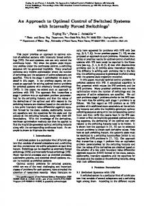
Figure 1: Feasible regions using Theorem 1 (“+”) and the proposed method with Corollary 3 (“∘”).

the modelling language YALMIP [18] with the solver SeDuMi [19]. Example 1

𝑇

𝑥 (𝑡) = [𝑥1 (𝑡) 𝑥2 (𝑡) 𝑥3 (𝑡)] , 𝑎 1 1 𝐴 (𝛼) = [0 35 𝑏] , [ 0 1 0]

1 𝐵 = [0] , [1]

13 1 1 0 35 𝑏 0 1 0

−0.5

with 𝑎 ≤ 𝑎 ≤ 0 and −1 ≤ 𝑏 ≤ 𝑏, where 𝑎 and 𝑏 are constant ̂ uncertain parameters. As the matrix 𝐵(𝛼) is uncertain, one defines a new state variable 𝑥3 (𝑡) = 𝑢(𝑡) = ∫ V(𝑡)𝑑𝑡. Thus, ̇ = V(𝑡) and one obtains the following extended 𝑥3̇ (𝑡) = 𝑢(𝑡) system [

̂ (𝛼) 𝐵̂ (𝛼) 𝑥̂ (𝑡) 0 ̂̇ (𝑡) 𝐴 𝑥 ] + [ 2×1 ] V, ]=[ ][ 1 𝑥3 (𝑡) 01×2 0 𝑥3̇ (𝑡)

(38)

or equivalently, 𝑥̇ (𝑡) = 𝐴 (𝛼) 𝑥 (𝑡) + 𝐵V,

(35)

(39)

where 𝑇

𝑥 = [𝑥1 (𝑡) 𝑥2 (𝑡) 𝑥3 (𝑡)] , 𝑎 1 1 𝐴 (𝛼) = [35 −1 𝑏] , [ 0 0 0]

[𝐴 1 𝐴 2 𝐴 3 𝐴 4] 𝑎 1 1 0 35 −36 0 1 0

−1

Figure 2: Feasible regions using Theorems 1 and 6 (“+”) and the proposed method with Corollary 3 and Theorem 6 (“∘”).

with 𝑎 ≤ 𝑎 ≤ 13 and 𝑏 ≤ 𝑏 ≤ −36, where 𝑎 and 𝑏 are constant uncertain parameters. Thus, the uncertain matrix 𝐴(𝛼) belongs to the polytope of vertices:

𝑎 1 1 = [ 0 35 𝑏 [0 1 0

−1.5 𝑎

Case 1. Stability. Consider the uncertain linear system given by (17), where

−2

13 1 1 0 35 −36 ] . 0 1 0 ] (36)

For the feasibility study, it was considered that the parameters 𝑎 and 𝑏 belong to the intervals 0 ≤ 𝑎 ≤ 10 and −97 ≤ 𝑏 ≤ −90, and 𝐵𝑖 = 𝐵, 𝑖 = 1, 2, 3, 4. In this example, the idea is to show that, considering only the stability, the methodology presented in this paper (Corollary 3) can be more efficient than the methodology used in the literature (Theorem 1). For this, it is sufficient to note that the region of feasibility using Corollary 3 is greater than the region obtained by using the Theorem 1, as shown in Figure 1. Example 2 Case 2. Stability and constraint on the norm of the controller gains. Consider the uncertain linear system given in (23), where

0 𝐵 = [0] . [1]

(40)

Therefore, the matrix 𝐴(𝛼) belongs to the polytope of vertices: [𝐴 1 𝐴 2 𝐴 3 𝐴 4] 𝑎 1 1 = [ 35 −1 𝑏 [0 0 0

𝑎 1 1 35 −1 −1 0 0 0

0 1 1 35 −1 𝑏 0 0 0

0 1 1 35 −1 −1 ] . 0 0 0] (41)

For the feasibility study, it was considered that the parameters 𝑎 and 𝑏 belong to the intervals −2 ≤ 𝑎 ≤ −0.5, −0.5 ≤ 𝑏 ≤ 1 and 𝐵𝑖 = 𝐵, 𝑖 = 1, 2, 3, 4. In control problems, it is important to consider performance indices, for instance, restrictions on the norm of the controller gains. Thus, to find the regions of feasibility of the system, Theorem 1 and Corollary 3 were used together with Theorem 6 in order to ensure stability and constraint in the control input. For the constraint on the norm of the control input, 𝜂 = 1600 and 𝜂𝑥 = 2 were fixed. From Figure 2, it can be observed that the proposed method is more flexible, since its feasible area is greater than that provided by Theorem 1.

𝑇

𝑥̂ (𝑡) = [𝑥1 (𝑡) 𝑥2 (𝑡)] , ̂ (𝛼) = [ 𝑎 1 ] , 𝐴 35 −1

1 𝐵̂ (𝛼) = [ ] , 𝑏

Example 3 (37)

Case 3. Stability, decay rate, and constraint on the norm of the controller gains.


𝑏

−5 −6 −7 −8 −9 −20

7

7. Switched Control Design of a Magnetic Levitator −15

−10

0

−5

5

10

15

To illustrate, the control of a magnetic levitator is designed, whose mathematical model [17, page 24] is given by:

𝑎

Decay rate 𝛽

Figure 3: Feasible regions using Theorems 4 and 6 (“+”) and the proposed method with Theorems 5 and 6 (“∘”).

6 4 2 0

0

5

10

𝑚𝑦̈ = −𝑘𝑦̇ + 𝑚𝑔 −

[𝑥1

Consider that during 𝑥2 ]𝑇 ∈ 𝐷, where

0 𝐵 (𝛼) = [ ] , 𝑏

(42)

with −27 ≤ 𝑎 ≤ 𝑎 and −10 ≤ 𝑏 ≤ 𝑏, where 𝑎 and 𝑏 are constant uncertain parameters that belong to the intervals −20 ≤ 𝑎 ≤ 15 and −9 ≤ 𝑏 ≤ −5, 𝑢 = 𝑢 − 𝑢0 and 𝑢0 > 0 the uncertain reference signal. Note that 𝐵(𝛼) is not constant and can be written as follows: 𝐵(𝛼) = 𝐵𝑔(𝛼), with 𝑔(𝛼) > 0, where 𝐵 = [0 − 1]𝑇 and 𝑔(𝛼) = −𝑏. Thus, the problem lies in the conditions of Case 3. As in previous examples, the region of feasibility of the system will be found, and in this case, Theorems 4 and 5 will be used along with Theorem 6, thus ensuring decay rate and constraint on the norm of the controller gains. Therefore, the vertices of the polytope, 𝐴 1 = 𝐴 2 , 𝐴 3 = 𝐴 4 , 𝐵1 = 𝐵3 , and 𝐵2 = 𝐵4 , are as follows: 0 1 𝐴 1,2 = [ ], 𝑎 −1 𝐵1,3

0 = [ ], 𝑏

0 1 𝐴 3,4 = [ ], −27 −1 𝐵2,4

0 =[ ]. −10

(43)

For the simulation of the feasibility region was specified in Theorems 4 and 5 a decay rate greater than or equal to 3 and in Theorem 6, the constraint on the norm of the controller gains by adopting 𝜂 = 400 and 𝜂𝑥 = 2. Thus, from Figure 3 one observes that the proposed method has a less conservative feasible region than that obtained with Theorem 4, which shows its flexibility.

(44)

the

required

(45)

operation,

𝑇

𝐷 = {[𝑥1 𝑥2 ] ∈ R2 : 0 ≤ 𝑥1 ≤ 0.15} .

Consider the uncertain linear system given in (3), where

0 1 ], 𝑎 −1

,

𝜆𝜇𝑖2 𝑘 𝑥̇ 2 = 𝑔 − 𝑥2 − . 2 𝑚 2𝑚(1 + 𝜇𝑥1 )

Figure 4: Feasible regions using Theorems 4 and 6 (“+”) and the proposed method with Theorems 5 and 6 (“∘”).

𝐴 (𝛼) = [

2

𝑥̇ 1 = 𝑥2 ,

Constraint on the controller gains 𝜂

𝑇

2(1 + 𝜇𝑦)

where 𝑚 is the mass of the ball; 𝑔 = 9.8 m/s2 is the gravity acceleration; 𝜇 = 2 m−1 , 𝜆 = 0.460 H, and 𝑘 = 0.001 Ns/m are constant parameters of the levitator; 𝑖 is the electric current; and 𝑦 is the position of the ball. Define the state variables 𝑥1 = 𝑦 and 𝑥2 = 𝑦.̇ Then, (44) can be written as follows [26]:

15

𝑥 (𝑡) = [𝑥1 (𝑡) 𝑥2 (𝑡)] ,

𝜆𝜇𝑖2

(46)

The goal of the simulation is to design a controller that keeps the ball in a desired position 𝑦 = 𝑥1 = 𝑦0 . Thus, the equilibrium point of the system (45) is 𝑥𝑒 = [𝑥1𝑒 𝑥2𝑒 ]𝑇 = [𝑦0 0]𝑇 . From the second equation 𝑥̇ 2 in (45), observe that in the equilibrium point, 𝑥̇ 2 = 0 and 𝑖 = 𝑖0 , where 𝑖0 = √(2𝑚𝑔/𝜆𝜇)(1 + 𝜇𝑦0 )2 . Linearizing the system (45) around the equilibrium point 𝑥 = 𝑥𝑒 , one has 0 0 1 𝑥̇ 𝑘 ] [𝑥1 ] + [ √2𝜆𝜇𝑔 ] 𝑢, [ 1 ] = [ 2𝑔𝜇 − 𝑥2 𝑥2̇ − [ 1 + 𝜇𝑦0 𝑚 ] [ √𝑚 (1 + 𝜇𝑦0 ) ] (47) where { 𝑥1 = 𝑥1 − 𝑦0 , { 𝑥1 = 𝑥1 + 𝑦0 , = 𝑥 , 𝑥 󳨐⇒ 2 2 { { 𝑥2 = 𝑥2 , { 𝑢 = 𝑖 − 𝑖0 , { 𝑖 = 𝑢 + 𝑖0 , 𝑥̇ 1 = 𝑥1̇ , { { { { 𝑥̇ 2 = 𝑥2̇ , 󳨐⇒ { 2𝑚𝑔 { 2 { { 𝑖=𝑢+√ (1 + 𝜇𝑦0 ) . 𝜆𝜇 {

(48)

Consider the constant position 𝑦0 varying is in the range 0.04 ≤ 𝑦0 ≤ 0.11 and that the mass 𝑚 is uncertain and belongs to the interval 0.02 ≤ 𝑚 ≤ 0.08, with 𝑥1 = 𝑥1 − 𝑦0 . Thus, from (46), the domain of the linear system (47) is 𝑇

𝐷2 = {[𝑥1 𝑥2 ] ∈ R2 : −0.11 ≤ 𝑥1 ≤ 0.11, 0.04 ≤ 𝑦0 ≤ 0.11, 0.02 ≤ 𝑚 ≤ 0.08} .

(49)

8

Mathematical Problems in Engineering Observe that the system (47) can be written as in (29); that

is, 𝑥̇ = 𝐴 (𝛼) 𝑥 + 𝐵𝑔 (𝛼) 𝑢,

(50)

𝑇

where 𝐵 = [0 − 1] and 𝑔(𝛼) = 𝑔(𝑚, 𝑦0 ) = √2𝜆𝜇𝑔/√𝑚(1 + 𝜇𝑦0 ). Note that 𝑔(𝛼) > 0, for all 𝑚, 𝑦0 ∈ 𝐷2 . Considering the domain 𝐷2 and the presented parameters of the levitator, one has the following vertices of the polytope for the system (47): 𝐴1 = 𝐴2 = [

0 1 ], 36.2963 −0.0125

𝐴3 = 𝐴4 = [ 𝐴5 = 𝐴6 = [

√(2𝑚𝑔/𝜆𝜇)(1 + 𝜇𝑦0 )2 , it follows that max {𝑖0 (𝑚, 𝑦0 )} = 1.5927,

𝑚,𝑦0 ∈𝐷2

min {𝑖0 (𝑚, 𝑦0 )} = 0.7050.

(53)

𝑚,𝑦0 ∈𝐷2

0 1 ], 36.2963 −0.05

Thus, setting 𝜉 = 10−4 the control law (30) for the levitator is given by

0 1 ], 32.1311 −0.0125

𝐴7 = 𝐴8 = [

with the classical method (Theorems 4 and 6) and the proposed method (Theorems 5 and 6), respectively. As the controller gains have been found, to implement the control law (30) one must find the maximum and minimum values of 𝑢0 = 𝑖0 in the domain 𝐷2 given in (49). As 𝑖0 =

(51)

0 1 ], 32.1311 −0.05

𝑢(𝜎,𝜉) (𝑡) = 𝑖(𝜎,𝜉) (𝑡) − 𝑖0 ,

with 𝑖(𝜎,𝜉) (𝑡) = −𝐾𝜎 𝑥 (𝑡) + 𝛾𝜉 , (54)

where 𝐾𝑖 , 𝑖 ∈ K8 are given in (52), 𝑇

𝐵1 = 𝐵3 = 𝐵5 = 𝐵7 = [0 −27.8025] ,

𝐾𝜎 ∈ {𝐾1 , 𝐾2 , 𝐾3 , 𝐾4 , 𝐾5 , 𝐾6 , 𝐾7 , 𝐾8 } ,

𝑇

𝐵2 = 𝐵4 = 𝐵6 = 𝐵8 = [0 −12.3060] . Initially, the feasibility region of the decay rate by the constraint on the controller gains is found, that is, the vertices of the polytope, given in (51), used in Theorems 4 and 5 with decay rate greater than or equal to 𝛽, varying in the range 0 ≤ 𝛽 ≤ 6.5, and the LMIs that guarantee the constraint on the controller gains, given in Theorem 6, with 0 ≤ 𝜂 ≤ 15 and 𝜂𝑥 = 10. As seen in Figure 4, the proposed method (Theorems 5 and 6) is more flexible than the method presented in the literature (Theorems 4 and 6). Fixing the parameters related to decay rate in 𝛽 = 5 and constraint on the controller gains, 𝜂 = 7 and 𝜂𝑥 = 10, the following gains and symmetric positive definite matrices were obtained: 𝐾 = [−8.9515 −1.3708] , 𝑃=[

7.4262 1.1192 ], 1.1192 0.1852

𝐾1 = [−12.9904 −2.1058] , 𝐾2 = [−14.0305 −2.2765] , 𝐾3 = [−13.0763 −2.1208] , 𝐾4 = [−13.9741 −2.2677] , 𝐾5 = [−13.9571 −2.2647] , 𝐾6 = [−15.6959 −2.5472] , 𝐾7 = [−14.2103 −2.3061] , 𝐾8 = [−15.4792 −2.5121] , 𝑃=[

6.7571 1.0964 ], 1.0964 0.1809

(52)

𝜎 = arg min {−𝑥(𝑡)𝑇 𝑃𝐵𝐾𝑖 𝑥 (𝑡)} , 𝑖∈K8

1.5927, { { 𝛾𝜉 = {−4438.723𝑥𝑇 𝑃𝐵 + 1.1488, { {0.7050,

if if if

𝑥𝑇 𝑃𝐵 < −𝜉, 󵄨󵄨 𝑇 󵄨󵄨 󵄨󵄨󵄨𝑥 𝑃𝐵󵄨󵄨󵄨 ≤ 𝜉, 𝑥𝑇 𝑃𝐵 > 𝜉.

(55)

For the numerical simulation, at 𝑡 = 0 s it considered the initial condition 𝑥(0) = [0.05 0]𝑇 , 𝑚 = 0.08 Kg, and 𝑦0 = 0.09 m. Thus, 𝑥(0) = 𝑥(0) − [𝑦0 0]𝑇 = [−0.04 0]𝑇 . In 𝑡 = 1 s, from Figure 5, the system is practically at the point 𝑥(1) = [𝑥1 (1) 𝑥2 (1)]𝑇 = [0.09 0]𝑇 . After changing 𝑚 from 0.08 Kg to 𝑚 = 0.04 Kg and 𝑦0 from 0.09 m to 0.05 m at 𝑡 = 2 s, one can see that the system is practically at the point 𝑥(2) = [0.05 0]𝑇 , which will be the new initial condition. Finally, changing 𝑚 from 0.04 Kg to 0.05 Kg and 𝑦0 from 0.05 m to 0.08 m for 𝑡 ≥ 2 s. Thus, as seen in Figure 5, 𝑥(∞) = [0.08 0]. Figure 5 illustrates the system response. Note that the control law given in (30) and (31) ensures that the system (47) is uniformly ultimate bounded, where 𝑦0 and 𝑚 are uncertain parameters and belong to the intervals 0.04 ≤ 𝑦0 ≤ 0.11 and 0.02 ≤ 𝑚 ≤ 0.08. Moreover, as can be seen in Figure 5, the new controller design presented in this paper is more efficient than the design commonly used in the literature. Note also that for certain values of the decay rate 𝛽 and the constraint on input 𝜂 such as 𝛽 = 6 and 𝜂 = 10, the controller (30) can be designed and the controller (4) cannot be designed, as shown in Figure 4. Observe that the function 𝛾𝜉 , given in (31), is important to ensure the uniform ultimate boundedness of the system and smoothness of the control input. Note that when 𝜉 is equal to zero, the function 𝛾𝜉 is a discontinuous function, and therefore the control input can also be discontinuous, as shown in Figure 6. Thus, the designer must choose 𝜉 according to the requirements.

0.09 0.07 0.05

9

𝑥2 (𝑡)

𝑥1 (𝑡)


0

1

2

3

4

5

6

0.2 0 −0.2

1

0

2

3

𝑡 (s)

4

5

6

𝑡 (s) (b)

𝑖 (𝑡)

(a) 2 1 0

1

0

2

3

4

5

6

𝑡 (s) (c)

0.08 0.06

𝑥2 (𝑡)

𝑥1 (𝑡)

Figure 5: Position 𝑦(𝑡) = 𝑥1 (𝑡), velocity 𝑥2 (𝑡), and electric current 𝑖(𝑡) of the controlled system, using the switched controller (30)-(31) (continuous line) and the classic controller (4) (dotted line), considering 𝑦0 = 0.09 m and 𝑚 = 0.08 Kg, and 𝑦0 = 0.05 m and 𝑚 = 0.04 Kg, 𝑦0 = 0.08 m and 𝑚 = 0.05 Kg, for 𝑡 ∈ [0, 2), 𝑡 ∈ [2, 4), and 𝑡 ≥ 4 s, respectively, with decay rate 𝛽 = 5, constraint on controller gains 𝜂 = 7 and 𝜂𝑥 = 10 and 𝜉 = 10−4 .

0

1

2

3

4

5

6

0.2 0 −0.2

1

0

2

3

𝑡 (s)

4

5

6

𝑡 (s) (b)

𝑖 (𝑡)

(a) 2 1 0

0

1

2

3

4

5

6

𝑡 (s) (c)

Figure 6: Position 𝑦(𝑡) = 𝑥1 (𝑡), velocity 𝑥2 (𝑡), and electric current 𝑖(𝑡) of the controlled system, using the switched controller (30)-(31), considering 𝑦0 = 0.09 m and 𝑚 = 0.08 Kg, 𝑦0 = 0.05 m and 𝑚 = 0.04 Kg, and 𝑦0 = 0.08 m and 𝑚 = 0.05 Kg, for 𝑡 ∈ [0, 2), 𝑡 ∈ [2, 4) and 𝑡 ≥ 4 s, respectively, with decay rate 𝛽 = 5, constraint on controller gains 𝜂 = 7 and 𝜂𝑥 = 10 and 𝜉 = 0.

8. Conclusions This paper proposed a new switched control design method for some classes of linear systems with polytopic uncertainties. In the proposed controller, the gain is chosen by a switching law that returns the smallest time derivative value of the Lyapunov function. The LMI used to find the gains are less conservative than that with only one state feedback gain [17], as seen in Figures 1 to 4. An application in the magnetic levitator control design illustrated the proposal. Thus, the authors believe that the proposed method can have useful practical applications on the control design of linear systems. Future studies on this subject include applications in power electronics [27].

[2]

[3]

[4] [5] [6]

Acknowledgments The authors would like to thank the Brazilian agencies CAPES, CNPq, and FAPESP which have supported this research.

[7]

[8]

References [1] M. A. Wicks, P. Peleties, and R. A. DeCarlo, “Construction of piecewise Lyapunov functions for stabilizing switched systems,”

[9]

in Proceedings of the 33rd IEEE Conference on Decision and Control, vol. 4, pp. 3492–3497, December 1994. D. Liberzon and A. S. Morse, “Basic problems in stability and design of switched systems,” IEEE Control Systems Magazine, vol. 19, no. 5, pp. 59–70, 1999. R. A. Decarlo, M. S. Branicky, S. Pettersson, and B. Lennartson, “Perspectives and results on the stability and stabilizability of hybrid systems,” Proceedings of the IEEE, vol. 88, no. 7, pp. 1069– 1082, 2000. J. P. Hespanha and A. S. Morse, “Switching between stabilizing controllers,” Automatica, vol. 38, no. 11, pp. 1905–1917, 2002. Z. Sun and S. S. Ge, “Analysis and synthesis of switched linear control systems,” Automatica, vol. 41, no. 2, pp. 181–195, 2005. A. Feuer, G. C. Goodwin, and M. Salgado, “Potential benefits of hybrid control for linear time invariant plants,” in Proceedings of the American Control Conference (ACC ’97), vol. 5, pp. 2790– 2794, June 1997. N. H. Mcclamroch and I. Kolmanovsky, “Performance benefits of hybrid control design for linear and nonlinear systems,” Proceedings of the IEEE, vol. 88, no. 7, pp. 1083–1096, 2000. H. Ishii and B. A. Francis, “Stabilizing a linear system by switching control with dwell time,” IEEE Transactions on Automatic Control, vol. 47, no. 12, pp. 1962–1973, 2002. D. J. Leith, R. N. Shorten, W. E. Leithead, O. Mason, and P. Curran, “Issues in the design of switched linear control systems:

10

[10]

[11]

[12]

[13]

[14]

[15]

[16]

[17]

[18]

[19]

[20]

[21]

[22]

[23]

[24]

[25]

Mathematical Problems in Engineering a benchmark study,” International Journal of Adaptive Control and Signal Processing, vol. 17, no. 2, pp. 103–118, 2003. S. Pettersson, “Controller design of switched linear systems,” in Proceedings of the American Control Conference (AAC ’04), vol. 4, pp. 3869–3874, Boston, Mass, USA, July 2004. H. Lin and P. J. Antsaklis, “Stability and stabilizability of switched linear systems: a survey of recent results,” IEEE Transactions on Automatic Control, vol. 54, no. 2, pp. 308–322, 2009. J. C. Geromel and G. S. Deaecto, “Switched state feedback control for continuous-time uncertain systems,” Automatica, vol. 45, no. 2, pp. 593–597, 2009. N. Otsuka and T. Soga, “Quadratic stabilizability for polytopic uncertain continuoustime switched linear systems composed of two subsystems,” International Journal of Control and Automation, vol. 3, no. 1, pp. 35–42, 2010. G. S. Deaecto, J. C. Geromel, and J. Daafouz, “Switched state-feedback control for continuous time-varying polytopic systems,” International Journal of Control, vol. 84, no. 9, pp. 1500–1508, 2011. D. Xie and M. Yu, “Stability analysis of switched linear systems with polytopic uncertainties,” in Proceedings of the IEEE International Conference on Systems, Man and Cybernetics (SMC ’06), vol. 5, pp. 3749–3753, October 2006. G. Zhai, H. Lin, and P. J. Antsaklis, “Quadratic stabilizability of switched linear systems with polytopic uncertainties,” International Journal of Control, vol. 76, no. 7, pp. 747–753, 2003. S. Boyd, L. E. Ghaoui, E. Feron, and V. Balakrishnan, Linear Matrix Inequalities in System and Control Theory, vol. 15, Society for Industrial and Applied Mathematics, Philadelphia, Pa, USA, 1994. J. Löfberg, “YALMIP: a toolbox for modeling and optimization in MATLAB,” in Proceedings of the 2004 IEEE International Symposium on Computer Aided Control System Design, pp. 284– 289, September 2004. J. F. Sturm, “Using SeDuMi 1.02, a MATLAB toolbox for optimization over symmetric cones,” Optimization Methods and Software, vol. 11-12, no. 1, pp. 625–653, 1999. J. Bernussou, P. L. D. Peres, and J. C. Geromel, “A linear programming oriented procedure for quadratic stabilization of uncertain systems,” Systems and Control Letters, vol. 13, no. 1, pp. 65–72, 1989. ˇ D. D. Siljak and D. M. Stipanović, “Robust stabilization of nonlinear systems: the LMI approach,” Mathematical Problems in Engineering, vol. 6, no. 5, pp. 461–493, 2000. R. Cardim, M. C. M. Teixeira, E. Assuncao et al., “Implementation of a DC-DC converter with variable structure control of switched systems,” in Proceedings of the IEEE International Electric Machines Drives Conference (IEMDC ’11), pp. 872–877, Niagara Falls, Canada, May 2011. R. Cardim, M. C. M. Teixeira, E. Assunçaõ et al., “Design and implementation of a DC-DC converter based on variable structure control of switched systems,” in 18th IFAC World Congress, vol. 18, pp. 11048–11054, Milan, Italy, 2011. B. R. Barmish, “Stabilization of uncertain systems via linear control,” IEEE Transactions on Automatic Control, vol. 28, no. 8, pp. 848–850, 1983. M. J. Corless and G. Leitmann, “Continuous state feedback guaranteeing uniform ultimate boundedness for uncertain dynamic systems,” IEEE Transactions on Automatic Control, vol. 26, no. 5, pp. 1139–1144, 1981.

[26] M. P. A. Santim, M. C. M. Teixeira, W. A. de Souza, R. Cardim, and E. Assunçaõ, “Design of a Takagi-Sugeno fuzzy regulator for a set of operation points,” Mathematical Problems in Engineering, vol. 2012, Article ID 731298, 17 pages, 2012. [27] R. Cardim, M. C. M. Teixeira, E. Assunçaõ, and M. R. Covacic, “Variable-structure control design of switched systems with an application to a DC-DC power converter,” IEEE Transactions on Industrial Electronics, vol. 56, no. 9, pp. 3505–3513, 2009.

Advances in

Operations Research Hindawi Publishing Corporation http://www.hindawi.com

Volume 2014

Advances in

Decision Sciences Hindawi Publishing Corporation http://www.hindawi.com

Volume 2014

Journal of

Applied Mathematics

Algebra

Hindawi Publishing Corporation http://www.hindawi.com


Volume 2014

Journal of

Probability and Statistics Volume 2014

The Scientific World Journal Hindawi Publishing Corporation http://www.hindawi.com


Volume 2014

International Journal of

Differential Equations Hindawi Publishing Corporation http://www.hindawi.com

Volume 2014

Volume 2014

Submit your manuscripts at http://www.hindawi.com International Journal of

Advances in

Combinatorics Hindawi Publishing Corporation http://www.hindawi.com

Mathematical Physics Hindawi Publishing Corporation http://www.hindawi.com

Volume 2014

Journal of

Complex Analysis Hindawi Publishing Corporation http://www.hindawi.com

Volume 2014

International Journal of Mathematics and Mathematical Sciences


Journal of

Mathematics Hindawi Publishing Corporation http://www.hindawi.com

Volume 2014


Volume 2014

Volume 2014


Volume 2014

Discrete Mathematics

Journal of

Volume 2014


Discrete Dynamics in Nature and Society

Journal of

Function Spaces Hindawi Publishing Corporation http://www.hindawi.com

Abstract and Applied Analysis

Volume 2014


Volume 2014


Volume 2014

International Journal of

Journal of

Stochastic Analysis

Optimization



Volume 2014

Volume 2014