qu' partir d'un arbre de preuves canonique, nous pouvons d river un pro- ... Mots clefs : Process, R seau de Petri, Logique Lin aire, Ordres partiels, Arbres de ...
Linear logic proofs and processes in Petri nets Jean Fanchon, Nicolas Rivière, Brigitte Pradin-Chézalviel, Robert Valette� LAAS-CNRS F-31077 Toulouse Cedex 4 {fanchon,nriviere,chezalvi,robert}@laas.fr Abstract
Equivalence between reachability in Petri nets and provability of certain sequent of linear logic has been proven in various ways. This work relates linear logic proofs based on the work of [13] to processes of Petri nets: we prove that from a canonical proof tree, an �équivalent� �nite process can be derived and reciprocally that for each �nite process, an�equivalent� canonical proof tree can be constructed. One of the main contributions of this article is that the decidability and e�ectiveness of linear logic sequent calculus in the multiplicative fragment used here can be used for determining the �nite processes of any Petri net. Keywords: Process, Petri nets, Linear logic, Partial orders, Proofs trees.
Résumé
L'équivalence entre accessibilité dans les réseaux de Petri et prouvabilité d'un certain séquent de logique linéaire a été prouvée de di�érentes manières. Ce travail porte sur les relations entre des preuves en logique linéaire basées sur [13] et les process de réseaux de Petri. Nous prouvons qu'à partir d'un arbre de preuves canonique, nous pouvons dériver un process �ni équivalent et réciproquement, pour chaque process �ni, un arbre de preuves canonique peut être construit. Une des contributions majeures de cet article est de montrer que l'e�cacité et la décidabilité du calcul des séquents en logique linéaire dans le fragment multiplicatif mis en ÷uvre ici peut être utilisé a�n de déterminer les process �nis d'un réseau de Petri. Mots clefs : Process, Réseau de Petri, Logique Linéaire, Ordres partiels, Arbres de preuves. � http://www.laas.fr/�robert
1
1 Introduction Various translations of a Petri net into linear logic [5] have been proposed. For some of them ([10, 8]), the transitions are considered as axioms which have to be added to linear logic. Important properties of the linear logic such as the cut elimination are then lost. However, it is in this context that the �rst relationships between linear logic proofs and partial orders (or concurrency between transition �rings) have been explored [8]. In [2], a Petri net is translated into a unique linear logic formula. In this way the structure of the Petri net is mixed with its initial marking [6] and the possible linear logic derivations do not necessarily correspond to what is possible in a Petri net. In [3] a semantic approach is used and Petri nets are considered as models of linear logic. This approach has not been very fruitful because the classical Petri net properties could not be translated into linear logic. This paper is based on yet an other approach [6, 13] in which markings are denoted by monomial in � (logical atoms are tokens) and transition �rings by implicative formulas (Pre(t)(Post(t) where Pre(t) and Post(t) are monomials in �). A reachability problem between an initial marking M0 and a �nal marking Mn , by means of a list of transitions l, is expressed by a sequent which has to be proven. In this last approach, no axiom has to be added to linear logic and cut elimination is therefore preserved. The equivalence between reachability and provability remains valid [6] and proof trees can be derived in a canonical way by means of the iterative use of the rule for the left elimination of linear implication (� (L rule�) [13] (one rule application for each transition �ring). Linear implication denotes causality between the consumed tokens and the produced ones. Each token, produced and consumed during the proof, corresponds to a precedence relation between two applications of the � (L rule� in the proof tree. In [13], these precedence relations are interpreted as precedence between the corresponding transition �rings in order to compute scenario duration. In fact, the set of precedence relations derived from a canonical proof tree de�nes a partial order over the set of transition �rings. On the other hand, processes and unfoldings of Petri nets constitute one of the main truly concurrent semantics for Petri nets ([12, 7, 1, 11, 9, 4]). The processes (�gure 1.b)(and unfoldings) of a Petri net for an initial marking, are �nite or in�nite bipartite acyclic graphs made up of places and transitions. In fact, in such nets (named occurrence nets), places denote tokens and transitions denote transition �rings. The unique input transition of each place corresponds to the �ring which has produced the corresponding token. A process is con�ict free, that is each place has a unique output transition denoting the �ring having consumed the corresponding token. In this paper we prove that, indeed, the sets of precedence relations derived from a canonical linear logic proof tree are �nite Petri net processes and reciprocally, that from each �nite process between an initial marking and a �nal marking a canonical proof tree of the sequent, made up of the corresponding markings and list of transitions, can be derived. One of the main contributions 2
of this result is that the decidability and e�ectiveness of linear logic sequent calculus in the multiplicative fragment used here ([5]) can be used for determining the �nite processes of any Petri net (bounded or not for example). The paper is organized in the following way. Section 2 details how Petri net reachability problems are encoded in the form of proofs of linear logic sequents and how canonical proof trees are derived. Section 3 reminds how processes can be derived from a Petri net and its initial marking, and presents two operations on processes used in sections 4 and 5. Section 4 shows how the set of precedence relations derived from a proof tree yields a �nite process between the initial and �nal markings of the sequent. Reciprocally, section 5 points out that from any �nite process, a proof tree proving the sequent composed of the initial marking, the �nal marking and a list of transition �rings corresponding to the transitions of the process. Finally section 6 discusses the results and give some hints for the future work.
2 Petri net reachability and linear logic After giving some notations, the translation of a reachability problem into the proof of a sequent of linear logic is presented. Finally the canonical proof tree is detailed.
2.1 Notations
A Petri net N ([14]) is a triple (S; T; W ) where S is a �nite set of places, T is a �nite set of transitions, such that S \ T = ;, and W : f(S � T ) [ (T � S )g ?! N is the �ow relation. X = S [ T is the set of the elements of N . The preset of a node x 2 X (written � x) is the set fy 2 X; W (y; x) 6= 0g and the postset of x (written x� ) is the set fy 2 X; W (x; y) 6= 0g. The set � x [ x� is denoted � x� . A marking M of N is a multiset M : S ?! N. Pre(t) and Post(t) are multisets of places such that 8s; t : Pre(t)(s) = W (s; t) and Post(t)(s) = W (t; s). Given two multisets of places M1 and M2 , we denote M1 v M2 the property 8s 2 S; M1 (s) � M2 (s). The reachability of M 0 from M by means of the �ring sequence � 2 T � (the elements of � are ordered) is denoted by: M [� > M 0.
2.2 Translation into linear logic
The Multiplicative Intuitionist fragment of linear logic (MILL) is su�cient for this approach. It only contains the multiplicative connectice � �� (conjunction of hypotheses) and the linear implication � (�. There is no negation and the meta connective � ;� is commutative. The speci�city of linear logic (with respect to classical logic) is that logical propositions are consumed when they are used for a deduction. Proving a sequent is verifying that the required hypotheses are available when they are used in a proof step. All the hypotheses have to be consumed in the same way as all the conslusion have to be produced. 3
s1 t1 s2 t3 s3 2
s1 t1 s2 t3 s3
�
�
t5 2
s7
s7
�
s4 t2 s5 t4 s6 a) Petri net
s7
s7
t2 s5 t4 s6 b) Process
s4
t5
s1 s1 s4 s4
Figure 1: A Process of a Petri net : example The atoms denotes tokens and their names are the places where they are located. Markings are denoted by monomial in �. Transition �rings are denoted by formulas of the form: t : Pre(t)(Post(t) (1) where Pre(t) and Post(t) are monomials in � (in the same way as markings). A reachability proof is expressed by the following sequent: M0 ; l0 ` Mn (2) where M0 is the initial marking, Mn is the �nal marking and l0 is an unordered list of formulas denoting transition �rings in the form of (1). These formulas indeed denote transition �rings because, if a transition t is �red n times to reach a marking, then the corresponding formula has to be present in n exemplars in l0 . The list l0 is a block of formulas connected by the meta connective � ;�. The fact that the proof of sequent 2, proves the reachability of Mn from M0 is a consequence of the equivalence between provability and reachability [6]. This paper can be seen as a re�nement of this result because it is proved that in addition to reachability, the processes between the two markings can be derived from the proof.
2.3 Example
Let us consider the Petri net fragment in �gure 1. The �rings of the transitions are denoted as follows: t1 : s1 �s7 (s2 �s7 t3 : s2 (s3 t2 : s4 �s7 (s5 �s7 t4 : s5 (s6 (3) t5 : s3 �s6 (s1 �s1 �s4 �s4 The reachability of a marking with two tokens in each of the places s1 and s4 and one token in the place s7 from a marking with one token in s1 , s4 and 4
s7 by �ring once transitions t1, t2, t3, t4 and t5 is denoted by the sequent: s|1 �s{z4 �s7}; |t1; t2; {z t3; t4; t5} ` s|1 �s1 �s{z4 �s4 �s7} (4) M0
Mn
l0
2.4 Proof of a sequent
A sequent proof tree is a syntactical proof. It is a set of rules. Each rule proves that a connective has been correctly introduced. The rules are given under the form of a tree which is read from the bottom (the sequent to be proven) to the top. The top leaves are identities. In the MILL fragment cuts can be eliminated (we recall that we do not add any proper axioms to linear logic for our translation) and in consequence it is always possible to rewrite a proof tree which only uses the rules concerning the connectives � and ( (plus the identity rule). In addition, as we have no linear implication in the right part of the sequent (it is a marking) we only need the rule concerning the left introduction of � (�. Let A be an atom, F , G and H be formulas and ? and � be blocks (lists of formulas connected by �,�). The rules involved in the proofs are the following ones: Proofs without cut can then be made by means of the following rules: Left introduction of (
Identity
? ` F �; G ` H ?; �; F G ` H
(
A ` A id (5)
(L
(6)
Right introduction of � Left introduction of � ?`F �`G � ?; F; G ` � � R ?; � ` F�G ?; F�G ` � L (8) (7) Let M = s1 ; s2; : : :; sn be a list of atoms (place names denoting tokens), we de�ne �(M) as the multiset of atoms M = �(M) with M (s) = jfi 2 [1; n] : si = sgj.
2.5 Canonical proof tree
Even with this restricted number of rules, a sequent can typically be proven by many proof trees. Taking advantage of the speci�c form of the sequents to be proven, we have elaborated a canonical way for constructing the proof trees.
2.5.1 Initial step Principle Starting from a sequent of the form of (2), the left introduction of � (rule 8) is applied iteratively until M0 is transformed into a list of atoms separated by commas. From a logic point of view, this means that these atoms can be used independently in the rules. Let M0 be this list (it is a block, 5
no longer a formula). We have : M0 = �(M0). The obtained sequent is M0 ; l0 ` Mn .
Example In the case of the sequent 4 we have (M0 = s1 ; s4; s7 , l0 = t1 ; t2; t3; t4; t5 and Mn = s1 �s1 �s4 �s4 �s7 ): s1 ; s4; s7 ; t1; t2; t3; t4; t5 ` s1 �s1 �s4 �s4 �s7 s1 ; s4�s7 ; t1; t2; t3; t4; t5 ` s1 �s1 �s4 �s4 �s7 �L �L (9) s �s �s ; t ; t ; t ; t ; t ` s �s �s �s �s 1
4
7 1 2 3 4 5
1
1
4
4
7
2.5.2 Iterative step Principle This step has to be executed once (and only once) for each tran-
sition �ring of the list l. It is applied on sequents which have the same form as (2) after the initial step that is:
Mi; li ` Mn
(10)
where Mi is a list of atoms delimited by commas, li is a list of transition �rings and Mn the �nal marking. It is decomposed into three substeps:
First substep The �rst substep is the application of the left introduction of ( (rule 6) for one selected transition �ring t of li . The current sequent of the proof is rewritten under the form of two sequents. Let us consider the notations in (6) with F = Pre(t) and G = Post(t). We restrict to the case in which ? is a sublist of Mi . The proof can only (it is in fact a necessary and su�cient condition because a sequent which is not well-balanced with respect to the atoms cannot be proven) be continued successfully if ? exactly contains the atoms in Pre(t) and with the same multiplicity. This is expressed by Pre(t) v �(?). Bloc � is made up of the remaining part of Mi concatenated with the remaining part of li after having deleted the formula corresponding to t. We have therefore the following construction for the considered transition �ring of t with Mi = ?; M0i and li = Pre(t)(Post(t); li+1 (note that Mi, M0i , ? and li+1 are blocks and Pre(t), Post(t) and Mn are formulas): ? ` Pre(t) M0 i ; Post(t); li+1 ` Mn ?; M0i ; Pre(t) Post(t); li+1 ` Mn
(
(L
(11)
Second substep The second substep consists in applying the rule 8 (�L) iteratively over G = Post(t) in order to transform this formula into a list of atoms. The derived sequent has the form of (10) where Mi+1 is derived from Mi by deleting in it the atoms of Pre(t) and by adding to it the atoms of Post(t) and li+1 is derived from li by deleting the formula corresponding to t. The right part of the sequent (Mn ) remains unchanged. 6
Third substep The third substep consist in applying the rule 7 (�R) iteratively over F = Pre(t) in order to obtain as many identity sequents as there was atoms in F . Then identity rule 5 is applied producing the leaves of the proof tree. Example Let us consider the proof of the sequent 4 again. If we consider transition �ring t1 we have the following proof tree fragment:
s1 ` s1 id s7 ` s7 id �R s2 ; s4; s7 ; t2; t3; t4; t5 ` Mn �L s1 ; s7 ` s1 �s7 s4 ; s2�s7 ; t2; t3; t4; t5 ` Mn s1 ; s4; s7 ; |s1 �s7 ( s � s 2 {z 7}; t2 ; t3; t4; t5 ` Mn t1
(L (12)
2.5.3 Final step Principle The �nal step (list li is empty) consists in applying iteratively rule �R in order to break down the sequent into a set of identities, and then to apply identity rules. This step is only possible if the last token list Mi contains exactly the tokens present in the �nal marking Mn . If it is not the case, the proof fails (which does not imply that the sequent is not provable).
Example Considering again the proof of the sequent 4, we have the following proof tree fragment: id s ; s :;:s: ` s �: :s: �s �R s ` s 1 1 4 4 7 4 4 7 �R s1 ` s1 id s1 ; s4; s4 ; s7 ` s1 �s4 �s4 �s7 �R (13) s1 ; s1; s4 ; s4; s7 ` s1 �s1 �s4 �s4 �s7
3 Petri nets processes
3.1 Causal nets and processes
A causal net [14] (also called deterministic occurence net [12, 1]) is an acyclic 1labelled 1-safe Petri net where any place has at most one input and one output transition. A process of a Petri net N is a causal net O associated with a bipartite graph morphism from O to N , i.e. a map mapping places on places, transitions on transitions, and satisfying some additional properties. In the present work, we consider only �nite Petri nets and processes. Formally causal nets and processes are de�ned as follows: A Causal Net is a Petri net O = (B; E; F ) such that: 1. F : B � E [ E � B ?! f0; 1g : transitions may produce (resp. consume) only single tokens into (resp. from) any single place. 7
2. 8e 2 E; � e 6= ; = 6 e� , i.e. any transition has at least one input and one output place. 3. 8b 2 B; j� bj � 1 and 8b 2 B; jb� j � 1: places are inputs and outputs of at most a single event. 4. F + is acyclic where F + � B [ E � B [ E is the transitive closure of F . A Process of a Petri net N = (S; T; W ) is a pair (O; �) where O = (B; E; F ) is a causal net, and � is a mapping � : B [ E ?! S [ T such that: 1. �(B ) � S , �(E ) � T : � maps the transitions (resp. the places) of O on the transitions (resp. the places) of N . 2. 8e 2 E : �(� e) = � �(e), �(e� ) = �(e)� : � preserves the presets and postsets of the transitions. V 3. 8e 2 E , 8s 2 S : W (s; �(e)) = j�?1 (s) \ � ej W (�(e); s) = j�?1(s) \ e� j : � preserves the input and output arities of the transitions. 4. Let Min be a marking of N , then (O; �) is a process of the marked V net (N; Min ) only if for any place s 2 S , Min (s) = jfb 2 B : � b = ; �(b) = sgj. This means that the initial places of O correspond bijectively to the tokens of the initial marking Min. In the following, (O; �) is a process of a marked net (N; Min ), with N = (S; T; W ) and O = (B; E; F ). A transition e 2 E is called an event and can be viewed as (an occurrence of) a �ring of the transition �(e) 2 T . A place b 2 B models a token in the place �(b) 2 S .
Remark 1 In processes, the �identities� of places and transitions, i.e. the sets
B and E , are not signi�cant, and we work up to sets bijections (or renaming). In particular in a canonical representation of a process, B could be de�ned by e� = [s2t� f(e; s)g � W (t; s), for any e 2 E with �(e) = t. For simplicity's sake we do not go here into the de�nitions of nets and processes morphisms and isomorphisms.
B-Cuts and reachable markings Let F � be the re�exive-transitive closure of F . Because F + is acyclic, F � (resp. F + ) is a partial order (resp. strict partial order) which we denote by �F (resp.