Linear programming-based directed local search for expensive multi-objective optimization problems: application to drinking water production plants F. Capitanescua,∗, A. Marvugliaa , E. Benettoa , A. Ahmadib , L. Tiruta-Barnab a
Luxembourg Institute of Science and Technology (LIST), Environmental Research and Innovation (ERIN) Department, 41 rue du Brill, L-4422, Belvaux, Luxembourg b University of Toulouse, INSA, UPS, INP, LISBP, 135 Avenue de Rangueil, F-31077 Toulouse, France
Abstract Local search (LS) is an essential module of most hybrid meta-heuristic evolutionary algorithms which are a major approach aimed to solve efficiently multi-objective optimization (MOO) problems. Furthermore, LS is specifically useful in many real-world applications where there is a need only to improve a current state of a system locally with limited computational budget and/or relying on computationally expensive process simulators. In these contexts, this paper proposes a new neighborhood-based iterative LS method, relying on first derivatives approximation and linear programming (LP), aiming to steer the search along any desired direction in the objectives space. The paper also leverages the directed local search (DS) method to constrained MOO problems. These methods are applied to the bi-objective (cost versus life cycle assessment-based environmental impact) optimization of drinking water production plants. The results obtained show that the proposed method constitutes a promising local search method which clearly outperforms the directed search approach. Keywords: OR in environment and climate change, Multi-objective optimization, Life cycle assessment, Environmental engineering, Expensive black-box model, Local search, Directed local search ∗
Corresponding author Email address:
[email protected] (F. Capitanescu)
Preprint submitted to European Journal of Operational Research
March 21, 2017
1. Introduction 1.1. Paper motivation, contribution, and organization The optimal design and operation planning of many industrial processes are intrinsically multi-objective optimization (MOO) problems (Deb, 2014). These latter typically involve conflicting goals and hence, in contrast to single objective optimization, exhibit a set of trade-off Pareto-optimal solutions. The increasingly accurate modeling of processes stemming from many real-world science and engineering fields lead to very complex MOO problems which preclude or make impractical the use of classical derivativebased mathematical programming approaches. This has given rise to a plethora of derivative-free meta-heuristic evolutionary global search (GS) algorithms (Zhou et al., 2011) such as: Non-dominated Sorting Genetic Algorithm (NSGA-II) (Deb et al., 2002), Strength Pareto Evolutionary Algorithm (SPEA2) (Zitzler et al., 2002), Multi Objective Evolutionary Algorithm based on Decomposition (MOEA/D) (Zhang & Li, 2007), multiobjective particle swarm optimization with multiple search strategies (Lin et al., 2015), etc. These basic GS algorithms are reliable and can explore challenging Pareto fronts. They are suitable for optimization over black-box simulators (or simulation optimization (Amaran et al., 2014)) of industrial processes and have been successfully applied to various practical engineering problems. However, their inherent slow convergence near to the optimum and the lack of an efficient termination criterion, motivated the development of various types of hybrid (or memetic1 ) algorithms (Ishibuchi & Murata, 1996, 1998; Knowles & Corne, 2000, 2005); the reader is refered to (Talbi, 2002; Raidl, 2006; Blum et al., 2011; Blum & Raidl, 2016) for comprehensive taxonomies of hybrid algorithms. The hybrid algorithms couple GS and local search (LS) along two schemes: • two distinct phases: GS attempts first to identify the most promising regions of the design space (exploration phase) and then its final solutions are passed to the LS for further local refinement (exploitation phase) (Deb & Goel, 2001); 1
This term has been first introduced in (Moscato et al., 1989).
2
• integrated approach: LS is embedded in the GS algorithm and called at a given pace to improve locally best solutions at hand (Ishibuchi & Murata, 1996, 1998; Knowles & Corne, 2000, 2005; Sindhya et al., 2013). The balance between exploration and exploitation, and in particular the effectiveness of the LS algorithm, are essential ingredients aimed at improving hybrid algorithm performance. For instance, LS can be very efficient obviously in the last stage of a problem as well as for unimodal problems while it can be less efficient at early stages for multimodal2 problems. This work focuses on LS methods and has as an additional motivation the fact that in many practical applications there is a need only to improve a current state of a system locally while, in many engineering fields, the computational budget is limited and/or the simulator is computationally expensive (Jones et al., 1998; Emmerich et al., 2002; Emmerich & Naujoks, 2004; Knowles & Corne, 2005; Emmerich et al., 2006; Santana-Quintero et al., 2010). The main contribution of this work is to devise a new neighborhoodbased iterative local search method, relying on first derivatives approximation and linear programming (LP). For comparison purposes the work also leverages the directed search (DS) method (Mej´ıa & Sch¨ utze, 2010; Sch¨ utze et al., 2010; Lara et al., 2013; Hern´andez et al., 2013) to constrained MOO problems. The remaining of the paper is organized as follows. The next subsection provides a literature review. Section 2 formulates conceptually the MOO problem and briefly describes the water production plant simulator, called EVALEAU. Section 3 describes both the proposed LS approach and the adapted directed search method. Section 4 provides optimization results with these approaches for a realistic model of a real-world drinking water production plant as well as for some benchmark test functions. Section 5 concludes. 1.2. Further literature review A) Local search. LS approaches for continuous optimization can be classified into two categories: • neighborhood-based (Deb & Goel, 2001; Igel et al., 2007) relying on Paretodominance relationship (Ikeda et al., 2001; Knowles & Corne, 2000), 2
I.e. a problem which exhibits more than one set of local Pareto-optimal solutions.
3
tabu search (Jaeggi et al., 2008), or composite functions e.g. simulated annealing (Serafini, 1994), hill climber technique (Deb & Goel, 2001), covariance matrix evolutionary strategy (Igel et al., 2007), etc. • directional (Harada et al., 2006; Lara et al., 2010; Kim & Liou, 2014; Mej´ıa & Sch¨ utze, 2010; Sch¨ utze et al., 2010; Lara et al., 2013; Hern´andez et al., 2013; Sch¨ utze et al., 2016). Two further classes of directional local search methods can be distinguished: (i) those which search dominating solutions along an arbitrary descent direction at hand (e.g. Pareto descent method (Harada et al., 2006), hill climber with sidestep (Lara et al., 2010), quadratic fitting adaptive efficient local search (Kim & Liou, 2014)) and (ii) those which aim at steering the search along a desired direction in the objective space (Mej´ıa & Sch¨ utze, 2010; Sch¨ utze et al., 2010; Lara et al., 2013; Hern´andez et al., 2013; Sch¨ utze et al., 2016). The latter class imposes a more constraining requirement than producing only dominating solutions along a given direction (which is anyway an ambitious goal) as in the former class. Furthermore it has an important advantage i.e. the ability to maintain the search along a given direction in the objective space which aids thereby preserving solutions spread (e.g. especially in a hybrid algorithm with two distinct phases). B) Consideration of environmental impact on optimization. The MOO of various industrial processes which further consider the LCA-based environmental impact has been extensively investigated (Jacquemin et al., 2012). When an approximate analytical model of the process can be developed, one can resort to mature mathematical programming methods such as: LP (Azapagic & Clift, 1999), nonlinear programming (NLP) (Gebreslassie et al., 2009), mixed-integer linear programming (MILP) (You et al., 2012), mixedinteger nonlinear programming (MINLP) (Yue et al., 2013; Guill´en-Gos´albez & Grossmann, 2010). However, comparatively less research effort has been devoted to the LCA-based MOO of drinking water production plants: e.g. (Capitanescu et al., 2015b) examines the performances of global optimizers (e.g. SPEA2 and NSGA-II) for the cost vs LCA-based environmental impact optimization, and (Ahmadi & Tiruta-Barna, 2015) proposes a hybrid algorithm combining GS algorithm NSGA-II and LS algorithm COBYLA for the cost vs LCAbased environmental impact vs water quality optimization. C) Optimization over expensive simulators. Due to their evolutionary features, both the basic GS and hybrid algorithms mentioned previously are 4
in principle not suitable for stringent real-world requirements (i.e. computationally expensive simulators and limited computational budget) because they may not satisfactorily progress toward the Pareto front. Such computationally expensive MOO problems with limited number of simulator calls constitute a class of problems emerged3 in the last decade and which requires algorithms with different accuracy/speed trade-offs. The few existing approaches (Santana-Quintero et al., 2010) in this research field aim at building computationally cheap surrogate models (Kleijnen, 2017) relying on (i) a single surrogate model e.g. Kriginig-based4 (Emmerich et al., 2002; Emmerich & Naujoks, 2004; Knowles, 2006; Emmerich et al., 2006; Zhang et al., 2010; Binois et al., 2015; Mlakar et al., 2015), radial basis functions (Regis, 2014), response surface approximation (e.g. MILP or NLP) proxies (Goel et al., 2007; Wanner et al., 2008; Capitanescu et al., 2015a), or (ii) hybrid algorithms e.g. surrogate-assisted evolutionary computation, in which the surrogate model uses radial basis functions (Regis, 2014) or ensemble5 (Lim et al., 2010) among others. 2. Multi-objective optimization over expensive simulators 2.1. MOO problem conceptual formulation The MOO problem corresponding to a representative operating scenario of a drinking water plant can be compactly formulated as follows: min
{f1 (x1 , . . . , xn ); f2 (x1 , . . . , xn )}
(1)
s.t.
gl (x1 , . . . , xn ) = 0, l = 1, . . . , q hk (x1 , . . . , xn ) ≥ hk , k = 1, . . . , c xi ≤ xi ≤ xi , i = 1, . . . , n,
(2) (3) (4)
x1 ,...,xn
where all functions involved (i.e. f1 , f2 , gl , and hk ) depend on the outcome of the drinking water production plant simulator EVALEAU, which is described in section 2.2. 3
This class was initiated in the context of single objective optimization (Jones et al., 1998) via the Kriging-based efficient global optimization (EGO) algorithm. 4 These methods are also named as Gaussian stochastic process modelling or Gaussian random field metamodels. 5 I.e. a combination of various surrogate models (e.g. polynomial regression, Gaussian process, etc.) aimed at offsetting the potential approximation error of a single surrogate.
5
In this formulation x = [x1 , . . . , xn ] is the vector of decision variables (e.g., design and operational parameters of the various plant unit processes), the objective f1 models the operational cost of the water plant (e.g., costs of raw materials, chemicals, electricity, etc.), the objective f2 models the LCA-based environmental impact of the plant. Equality constraints (2) model the set of equations which describe the input-output mass flow for each unit process in the whole chain. These equations are enforced intrinsically by the simulator. Inequality constraints (3) enforce outlet water drinkability quality, according to the best water quality class (SEQEau, 2003), modeled by a set of seven major aggregated parameters6 . Inequality constraints (4) represent physical bounds of the decision variables. Let us emphasize that, tackling the MOO problem (1)-(4) by means of classical mathematical programming methods is impractical, if feasible at all, because constraints (2)-(3) possess challenging features such as: nonlinearity, non-convexity, reliance on the expert program PHREEQC for simulating chemical reactions equilibrium in some unit process (being thereby very difficult to fully express in analytical form) among others. 2.2. EVALEAU simulator For the sake of completeness we provide in this subsection a description of the EVALEAU simulator taken from (Capitanescu et al., 2015a). “The EVALEAU simulator is a state-of-the-art process modelling - LCA tool for prospective and retrospective simulation of potable water treatment chains (M´ery et al., 2013). The simulator comprises a certain number of unit processes (UPs) for water treatment which can be combined to simulate a specific treatment chain (see Fig. 1). The simulator was developed in the LCA software Umbertor , relies on the software PHREEQC(Parkhurst & Appelo, 2013) for the model of chemical reactions in aqueous solutions, and is linked to the Ecoinventr database (Weidema et al., 2013) for the life cycle inventory (LCI) of background processes. “The UP modules are mathematical models consisting mainly of a set of equations defining energy and mass balances. They can represent the removal of pollutants via chemical reactions (precipitation, coagulation, and 6
E.g. total coliforms, total trihalomethanes, total organic carbon, Escherichia coli, faecal streptococci, turbidity, and conductivity.
6
Figure 1: Flowchart of the potable water production plant used in the case study (Capitanescu et al., 2015a).
oxidation), separation (settling, filtration, etc.), elimination of microbiologic pathogens, and other treatments such as mineralization and softening to correct water quality. The modelling parameters for the different UPs include engineering design choices (i.e. device hydrodynamics, pipe diameter, efficiencies), technical issues (i.e. pumping height, backwashing schedule, filtering area, etc.), and legal restrictions (i.e. the disinfection requirement criteria)” (Ahmadi & Tiruta-Barna, 2015). The input of EVALEAU is the inlet (river) water, which quality is described by a set of “more than hundred criteria including parameters such as temperature, pH, turbidity, UV absorbance, dissolved organic carbon, pathogenic microorganisms, inorganic compounds, micro-pollutants, and reaction products” (Ahmadi & Tiruta-Barna, 2015). The outputs of the simulator are: the outlet treated water, which quality is described by the same set of parameters as the inlet water, the operation cost of the plant, and the LCI. EVALEAU-LCA considers the functioning stage of the plant life cycle and neglects the construction and decommissioning steps as explained in (M´ery et al., 2013). System boundaries correspond to cradle to gate analysis, i.e. all background processes are included. The functional unit chosen is set to 1m3 of potable water at the plant.” 7
f2 f20
C F(x0)
d1
A d2
d
P D
B f10
f1
Figure 2: Illustration of the directed search method goal in a bi-objective space.
3. The proposed LP-based local search method The proposed LP-based LS method is presented in a stand-alone fashion, while a preliminary discussion of its potential integration in a hybrid algorithm is provided in section 3.5. 3.1. Rationale Figure 2 sketches, in a two-dimensional objective space, the basic idea of DS method (Mej´ıa & Sch¨ utze, 2010; Sch¨ utze et al., 2010; Lara et al., 2013; Hern´andez et al., 2013), which inspired the proposed LP method. Specifically, the method attempts to generate, starting from a given initial point x0 = [x01 , x02 , . . . , x0n ] (and its corresponding image in the objective space F (x0 ) = [f10 = f1 (x0 ); f20 = f2 (x0 )]), a sequence of points whose images are located ideally along the desired direction d = [d1 ; d2] ∈ R2 in the objective space, converging eventually to the point P on the Pareto front. In most cases one typically looks for descent directions d able to improve both objectives, leading thereby to a sequence of dominating points moving toward the Pareto front. However, depending on the location of the initial point, the part of the Pareto front that can be explored by descent directions (i.e. the part between points A and B) may be small. Note that, the proposed LP method is not limited to descent directions but can explore the whole Pareto front (e.g. also the sets of points between A and C, and B and D, respectively) by generating a sequence of non-dominated points. Figure 3 shows intuitively the sequence of points (e.g. x0 , x1 , . . . , x7 ) generated by the LP local search around the current point at every iteration 8
x2max x20
x1 x3 x4
x0
x2
x5 x6
x2min x1min
x7
x10
x1max
Figure 3: Illustration in a two-dimensional parameter space of the sequence of points generated by the LP-based local search at each iteration starting from an initial point x0 = [x01 , x02 ].
within a neighborhood of fixed radius θ, according to constraint (16). 3.2. Computation of first derivatives approximation The proposed local search method relies on the computation of first derivatives approximation. This computation depends on the number of points available p and its relationship with the number of decision variables n. Three cases can be distinguished in practice as follows. 1. The case where n = p. Assuming that n different points x1 = [x11 , . . . , x1n ], . . ., xn = [xn1 , . . . , xnn ], have been evaluated (i.e. f11 = f1 (x1 ), . . . , f1n = f1 (xn ) are known) in the neighborhood of the initial point x0 = [x01 , . . . , x0n ], the first derivatives approximation of function f1 is computed by solving the following linear system of equations: f˜1x1 f11 − f10 x11 − x01 . . . x1i − x0i . . . x1n − x0n .. .. .. .. .. . = . . . ... . ... n 0 n 0 n 0 n 0 x1 − x1 . . . xi − xi . . . xn − xn f1 − f1 f˜1xn (5) ˜ ˜ ˜ where f1x1 , . . . , f1xi , . . . , f1xn is the approximation of the function f1 first derivatives with respect to the decision variables x1 , . . . , xi , . . . , xn . The first derivatives approximation of all functions involved in the MOO problem (e.g. f2 , hk , etc.) can be computed likewise. 9
2. The case where n > p. Since the number of unknowns is greater than the number of equations the linear system (5) is underdetermined (i.e. an infinite number of solutions satisfying the equations exists). In this case one picks the greedy solution which consists in computing the least squares of the first derivatives approximation by solving the following simple optimization problem: min
f˜1x1 ,...,f˜1xi ,...,f˜1xn
p X
[f1j − f10 −
j=1
n X
f˜1xi (xji − x0i )]2
(6)
i=1
subject to: f1j − f10 =
n X
f˜1xi (xji − x0i ), j = 1, . . . , p
(7)
i=1
3. The case where n < p. Because there are fewer unknowns than equations the linear system (5) is overdetermined. In this case one computes the first derivatives approximation via the least squares of the mismatches of the linear equations resorting to an unconstrained minimization problem: min
f˜1x1 ,...,f˜1xi ,...,f˜1xn
p X
[f1j
−
j=1
f10
−
n X
f˜1xi (xji − x0i )]2
(8)
i=1
3.2.1. Remarks Note that, although less exact, the proposed technique to approximate first derivatives has two major advantages compared to the classical approximation based on finite-differences: • it takes into account to some extent nonlinearity and interactions between decision variables; • it has a broader scope and computational advantages since it applies to a any given set of points at hand (fitting thereby very well in the hybrid algorithms strategy) while the classical gradient requires additional computational effort for functions evaluations by shifting one variable at the time from the initial point.
10
3.3. Formulation of the LP-based local search problem Let us first emphasize that, as explained in section 3.1 and illustrated Fig. 2, to enable the exploration of the entire Pareto front the proposed method adopts weights on objectives w = [w1 ; w2 ] rather than a descent direction d = [d1 ; d2 ] as in DS method. The LP local search method assumes a linear functions model in the search neighbourhood and can be formulated as a bi-objective constrained LP problem: min α + ρ[w1 (f1 − f 1 )/(f 1 − f 1 ) + w2 (f2 − f 2 )/(f 2 − f 2 )] xi ,α
s.t.
f1 =
f10
+
f2 = f20 + hk = h0k +
n X
i=1 n X
i=1 n X
(9)
f˜1xi (xi − x0i )
(10)
f˜2xi (xi − x0i )
(11)
˜ kx (xi − x0 ) ≥ h , k = 1, . . . , c h k i i
(12)
i=1
w1 (f1 − f 1 )/(f 1 − f 1 ) ≤ α
(13)
w2 (f2 − f 2 )/(f 2 − f 2 ) ≤ α xi ≤ xi ≤ xi , i = 1, . . . , n −θ(xi − xi ) ≤ xi − x0i ≤ θ(xi − xi ), i = 1, . . . , n
(14) (15) (16)
where, α is a real-valued variable, ρ is a very small positive value set to 10−6 , for function f1 (the notations associated to functions f2 and hk have likewise meaning): f10 is its initial value, f 1 and f 1 are its maximum and minimum value among the available points, the ratio (f1 − f 1 )/(f 1 − f 1 ) is used to normalize7 the objective in order to obtain an even spread of Pareto solutions, and θ is the radius of the neighborhood used for the local search (a single value of the radius, common for all decision variables, is assumed; however, one individual value per variable is also possible if deemed more advantageous in a given context). In this formulation the objective function (9) aims at minimizing the scalar α, which in turn minimizes, via the enforcement of constraints (13) and 7
Actually the value of this ratio will belong strictly to the interval [0;1] if the whole design space is considered.
11
(14), both objectives f1 and f2 along the desired search direction. Note that the objective (9) is also augmented with a second term, which has the role to avoid the convergence to a weak Pareto-optimal solution. The constraints (10), (11), and (12) are first derivatives approximation-based linearizations of functions f1 , f2 , and hk , k = 1, . . . , c, respectively, in the neighborhood of the initial point, constraints (13) and (14) aim at providing a solution located as close8 as possible to the desired objectives weights w = [w1 ; w2], where w1 , w2 ∈ [0; 1], constraints (15) impose physical bounds on decision variables, and constraints (16) model via the radius θ the neighborhood of the search. Note that an advantage of this method over the DS is its natural ability to explore the whole Pareto front via the choice of weights w1 and w2 likewise in classical aggregation method, while the DS has difficulties to explore extreme Pareto front points (i.e. when the problem becomes single objective), as argued in page 159 (Lara et al., 2013) and shown graphically in Figure 2 in (Sch¨ utze et al., 2010). 3.4. Algorithm of local search as an independent module The LS algorithm9 is intuitively illustrated in Fig. 3 and can be summarized as follows. • input: initial point x0 , the neighborhood radius θ (it is typically10 set to 0.1), weights vector w, and maximum number of iterations Jmax . • output: sequence of solutions generated at each iteration {xj }, j ∈ N. The algorithm performs at each iteration j = 1, . . . , Jmax the following steps: 1. Generate randomly and evaluate n points in the neighbordhood N (xj , θ) = {xj ∈ Rn |xj−1 − θ(xi − xi ) ≤ xi ≤ xj−1 + θ(xi − xi ), i = 1, . . . , n}. i i Note that this step takes advantage of the solutions (if any) belonging to this neighborhood already evaluated in the previous iterations. 8
If both constraints are binding at the optimum it means that under linearity assumptions the optimal solution is located on the desired search direction. 9 For the sake of presentation simplicity but without loss of generality we consider hereafter only the case where the number of points equals the number of decision variables (p = n) and hence the first derivatives approximation are computed according to (5). 10 An efficient determination of adaptive search region can be carried out along the approach proposed in (D¨achert et al., 2017).
12
2. Compute first derivatives approximation by solving the linear equations system (5). 3. Solve the LP problem (9)-(16). Let xj be its optimal solution. 4. Evaluate the new candidate solution xj . 5. If this new solution dominates the previous solution (i.e. xj ≺ xj−1 ) go to step 1. Otherwise launch a back-up procedure which consists in searching among the randomly generated solutions in the neighbourhood the best dominating one. If there is no dominating solution, then one searches the best non-dominated solution according to the composite objective (9). If there is no better non-dominated solution it means that all solutions in the current neighborhood are dominated by the solution in the previous iteration xj−1 and the algorithm stops. Otherwise set the solution produced by the back-up procedure as the new candidate solution xj and go to step 1. Note that the algorithm is not supposed to generate only dominating solutions as explained in section 3.1. The algorithm stops either after completing the maximum number of iterations Jmax or as all exiting solutions in a neighborhood are dominated by the solution in the previous iteration, which indicates the close proximity to the (at least local) Pareto front. The worst-case computational effort of the stand-alone algorithm is (n + 1) × Jmax , i.e. it scales linearly with the number of decision variables. However, in practice, a non-negligible (problem-dependent) computational effort can be saved thanks to the inherent overlapping of successive neighbourhoods (see Fig. 3) and the presence of already evaluated solutions in these overlapping areas. Furthermore, when embedded into a hybrid algorithm the best-case computational effort is null as explained hereafter. 3.5. Towards a hybrid algorithm combining global search and local search This section makes a first attempt to outline the potential integration of the proposed LP-based local search method into a hybrid algorithm (section 4 will bring some empirical evidence of its benefits) while the challenging goal of the full design of an efficient memetic algorithm integrating the proposed local search method requires further thoughts and is beyond the scope of this paper. The integration of the proposed LP-based local search method into a hybrid algorithm, in which the LS method can be used in two modes:
13
1. mode A: relying on the solutions already evaluated in the GS, requiring therefore practically free functions evaluation cost11 ; 2. mode B: using both the solutions already evaluated in the GS as well as generating independently new solutions in the LS module (but still taking advantage of points already existing in the various neighborhoods). The input data and output of the algorithm are the following: • input: number of points approximating the Pareto front m, set of weights {w1 , . . . , wm }, LS parameters (e.g. neighborhood minimum radius θ, maximum number of iterations Jmax ), and allowed overall computational budget B (number of evaluations) and its share among GS (BGS ) and LS (BLS = B − BGS ). Acknowledging that finding the optimal balance between exploration and exploitation is a delicate problem-dependent task (Ishibuchi et al., 2003), where generally BLS ∈ [0.05, 0.5]B, in this work we assume BLS = 0.2B. • output: m solutions approximating the Pareto set {x⋆j }, j = 1, . . . , m. For the sake of simplicity the potential hybrid algorithm is described hereafter in a two-phase sequential GS and LS framework The major steps of the potential hybrid algorithm are: 1. Run a global search algorithm (e.g. SPEA2, NSGA-II, etc.) for a predefined number of generations12 until the allowed GS budget BGS is exhausted. 2. Choose the best solutions for local search by mapping the GS algorithm current best solutions set13 with the set of weights {w1 , . . . , wm }. 3. As long as the allowed LS budget BLS is not exhausted, for j = 1, . . . , m do: (a) Pick the best solution xj corresponding to the weights vector wj . 11
Assuming that the time spent in solving the linear system (5) and the LP problem (9)-(16) is negligible compared to one expensive simulator call. 12 At least say 5-10 generations are required in order to feed the LS module with an acceptable number of solutions. 13 This set depends on the peculiarity of the GS algorithm and represents e.g. the current population in NSGA-II or the external archive in SPEA2. Note that only non-dominated solutions are selected, whose number may be lower than m.
14
(b) Build an adaptive radius neighborhood around xj , Na (xj , xr , θ) = {xj ∈ Rn | min{xri , xj−1 − θ(xi − xi )} ≤ xi ≤ max{xri , xj−1 + θ(xi − i i xi )}, i, r = 1, . . . , n}, which includes its n-closest solutions xr , r = 1, . . . , n evaluated in the GS. (c) Perform local search in the neighborhood Na (xj , xr , θ) according to the LS algorithm in section 3.4. Let x⋆j be the best solution obtained by the LS module. 3.6. Formulation of the constrained directed search (DS) approach The directed search algorithm, initially developed for unconstrained MOO (Mej´ıa & Sch¨ utze, 2010; Sch¨ utze et al., 2010; Lara et al., 2013; Hern´andez et al., 2013), is extended here to constrained MOO, specifically by considering operational constraints (21), physical limits on decision variables (22), and neighborhood boundaries (23). Assuming that p points xj have been evaluated (i.e. values of functions f1 (xj ), f2 (xj ), and hk (xj ) are known) in the neighborhood of the initial point x0 , the DS method computes the optimal adjustment of decision variables ∆x⋆ attempting to steer the search in the objective space along the desired direction d = [d1 , d2 ] by solving the following quadratic programming problem which searches for the least squares of the weights λj and thereby for a greedy optimal direction ∆x⋆ : min
p X
s.t.
p X f1 (xj ) − f1 (x0 )
λj = −d1
(18)
X f2 (xj ) − f2 (x0 )
λj = −d2
(19)
λj ,∆x
λ2j
(17)
j=1
j=1 p
j=1
∆x =
||xj − x0 ||2 ||xj − x0 ||2 p X
λj (xj − x0 )
(20)
j=1
hk (x0 ) +
p X
λj [hk (xj ) − hk (x0 )] ≥ hk , k = 1, . . . , c
(21)
j=1
x ≤ x0 + β∆x ≤ x −θ(x − x) ≤ β∆x ≤ θ(x − x) 15
(22) (23)
where λj is the weight corresponding to j-th direction of variables adjustments xj − x0 , and β is the minimum steplength (usually set to 10−4 ). The role of parameter β is very important, for instance to avoid cases in which a decision variable reaches a physical bound and the optimal direction points outside this bound which would lead to the search stuck. So this parameter ensures that a non-zero steplength in the optimal direction exists so that box constraints (22)-(23) are enforced. Note that, according to constraint (20), the direction of variables adjustments ∆x is a linear combination (weighted by λj ) of the p available directions xj − x0 . In order to ensure a fair comparison with the proposed LP-based method we also assume here that the linearization holds in the neighborhood of the initial point. Accordingly, the line search (Lara et al., 2013) for the optimal step along the optimal direction ∆x⋆ is not performed. Therefore, in this work, the solution produced by the DS procedure is xnew ← x0 + ∆x⋆ . 4. Numerical results 4.1. Brief description of the studied water plant and simulation tools The proposed optimization approaches are applied to a realistic model of an existing French water treatment plant. The treatment chain of the inlet river water contains the major unit process shown in Fig. 1 such as: pumping, two ozonation phases, coagulation/flocculation, settling, biolite filtration, granular activated carbon (GAC) filtration, and bleach disinfection. The simulations are run on a 2.70GHz/8GB computer. The EVALEAU simulator runs in Umbertor 5.6 environment and is linked to the Ecoinventr v2.2 LCI database for background processes. The linear programming problem (9)-(16) and the three quadratic programming problems (6)-(7), (8) and (17)-(23) are modeled in GAMS version 23.9 (McCarl, 2013) and solved via powerful solvers such as CPLEX and CONOPT respectively. The environmental impact metric focuses only on climate change impact category, e.g. Global Warming Potential (GWP) factors based on 100 yearstime horizon, and is computed using the Midpoint ReCiPe LCIA method (Goedkoop et al., 2009). The functional unit is set to 1m3 of potable water at the plant.
16
4.2. Experiments assumptions The numerical experiments and comparisons conducted hereafter rely on the following assumptions: • We consider a set of 6 continuous decision variables, namely: the ozone transfer efficiency and the pure oxygen fraction in feed gas in both ozonation unit processes (see Fig. 1), the coagulant dose in the coagulation/flocculation unit and the granular activated carbon (GAC) regeneration frequency in the GAC filtration unit. • To highlight the proposed method hybridization potential we use the state-of-the-art global meta-heuristic evolutionary algorithm SPEA2 (Zitzler et al., 2002). The algorithm is run with the default values proposed on PISA platform (Bleuler et al., 2003), using a population of 24 individuals. 4.3. SPEA2 vs MOEA/D Figure 4 provides the Pareto front approximation (after 10, 20, and 50 generations; the latter corresponds to the baseline Pareto front) obtained with SPEA2 and MOEA/D algorithms. MOEA/D algorithm is run with default settings, according to the Tchebycheff approach with normalized objectives and with a neighborhood size of 8 individuals. From this figure one can observe that while SPEA2 algorithm converges fast to the Pareto front, due to its intrinsic features, the MOEA/D algorithm progresses much slowlier and, even after 50 generations, the lower part of the Pareto front remains still unexplored. These results allow concluding that the popular algorithm MOEA/D is certainly appealing for MOO problems where the number of evaluations is not a concern, but is less appropriate for expensive MOO problems with limited resources as well as justify our preference toward SPEA2 algorithm as a MOO algorithm comparison baseline. 4.4. Impact of the number of points on the PG local search method performance We first investigate the influence of the number of points used to compute first derivatives approximation upon the performance of the LP-based method. For illustrative purposes the LP-based method is run in stand-alone mode for Jmax = 7 iterations. 17
10 generations 20 generations 50 generations
cost (monetary units)
0.054 0.052 0.05 0.048 0.046 0.044 0.16
0.18
0.2
0.22
0.24
0.26
0.28
0.3
climate change - GWP100 (kg. CO2-Eq)
(a) SPEA2 10 generations 20 generations 50 generations
cost (monetary units)
0.054 0.052 0.05 0.048 0.046 0.044 0.16
0.18
0.2
0.22
0.24
0.26
0.28
0.3
climate change - GWP100 (kg. CO2-Eq)
(b) MOEA/D Figure 4: Cost vs. environmental impact Pareto front approximation with SPEA2 and MOEA/D algorithms.
18
operational cost (monetary units)
0.062 0.06
Pareto front proposed method (6 points) proposed method (4 points)
0.058 0.056 0.054 0.052 0.05 0.048 0.046 0.044 0.16
0.18 0.2 0.22 0.24 0.26 0.28 climate change - GWP100 (kg. CO2-Eq)
0.3
Figure 5: Solution path obtained with the proposed LP-based method for 4 points and 6 points used to compute first derivatives approximation.
Fig. 5 shows the solution path obtained, starting from the initial operating point of the water production plant, with the LP-based local search method for 4 points and 6 points, as well as the Pareto front obtained with the SPEA2 algorithm. For the sake of figure legibility and because it suffices to conclude only the paths corresponding to the two ends of the Pareto front (i.e. the points corresponding to the minimum cost and the minimum environmental impact respectively) are shown. One can observe that the smaller number of points is insufficient in most iterations of the local search to steer the search along the desired direction and, in particular, the performance is poor for the cost minimization endpoint. On the other hand, using the larger number of points allows steadily steering the search path toward the Pareto end points. Other experiments conducted with the approach but not reported in the paper confirm these findings and hence, this example allows concluding that, in order to obtain the desired behavior, the LP-based method requires generally at least as many different points as decision variables or, in other words, it cannot take systematically advantage from a limited number of points (compared to the number of decision variables). Fig. 6 displays the solution path obtained with the PG method for 6 points and 8 points. Note that, considering the larger number of points leads to a slight improvement of solutions and also to a more steady steer 19
operational cost (monetary units)
0.062 0.06
Pareto front proposed method (6 points) proposed method (8 points)
0.058 0.056 0.054 0.052 0.05 0.048 0.046 0.044 0.16
0.18 0.2 0.22 0.24 0.26 0.28 climate change - GWP100 (kg. CO2-Eq)
0.3
Figure 6: Solution path obtained with the LP-based method for 6 points and 8 points used to compute first derivatives approximation.
of the search while with the smaller number of points one can sometimes temporarily exhibit a significant deviation from the desired search direction. As it will become clear later on, the same conclusions regarding the number of points needed to obtain the desired behavior from the local search hold for the DS method as well. Unless stated otherwise, in what follows we will run the LP-based method with the same number of points as the decision variables, i.e. 6 points. 4.5. LP-based method versus DS We assess the ability of LP-based and DS as stand-alone methods to steer the search into the desired direction in the objective space. The same number of 6 points is assumed for each method to ensure a fair comparison. One requires approximating the Pareto front by 24 solutions. 4.5.1. Starting from the midpoint The first comparison assumes starting from the midpoint, that is each decision variable is set to the half value of its physical range. The starting point corresponds to a cost of 0.0566 monetary units (euro/1m3 of treated water) and an environmental impact of 0.354 kg. CO2 -eq. Fig. 7 shows the solution path obtained with the DS local search method. One can remark that, although the solutions spread is acceptable, the DS 20
operational cost (monetary units)
0.06 0.058 0.056 0.054 0.052 0.05 0.048 0.046
Directed search Pareto front
0.044 0.15
0.2 0.25 0.3 0.35 climate change - GWP100 (kg. CO2-Eq)
0.4
Figure 7: Midpoint start: DS method solution path and approximated front.
method is unable to consistently steer the search along the desired direction and, at some iterations, the solutions proposed are dominated. In fact only around half among the final solutions move toward14 the Pareto front but do not approach it sufficiently close. This unsatisfactory behavior is attributable to the search hitting some constraints (especially in the latter stage of the search where one is closer to the Pareto front) which prevents the directed search to further progress toward the Pareto front. These results indicate that DS method seems useful mostly in the context in which it was primarily proposed, i.e. the unconstrained optimization (Lara et al., 2013). Fig. 8 shows the solution path obtained with the LP-based local search method. Note that the method presents a very good ability to steer the search along the desired direction. Except for a single trajectory (see the middle of the figure) which gets stuck at a larger distance to the Pareto front than the other trajectories, the method produces generally a very good approximation of the Pareto front (both as accuracy, the worst solution being only 3% suboptimal, and spread). In particular the upper concave part of the Pareto front is perfectly covered. 14
It was reported that DS is unable to explore the end points of the Pareto front (Lara et al., 2013)
21
operational cost (monetary units)
0.058
Pareto front proposed method
0.056 0.054 0.052 0.05 0.048 0.046
0.044 0.16 0.18 0.2 0.22 0.24 0.26 0.28 0.3 0.32 0.34 0.36 climate change - GWP100 (kg. CO2-Eq)
Figure 8: Midpoint start: LP-based method solution path and approximated front.
By looking at Figures 7 and 8 one can conclude that the LP-based method largely outperforms the DS method. 4.5.2. Starting from the plant initial operating point The starting point corresponds to the initial operating point of the water plant i.e. to a cost of 0.0566 monetary units and an environmental impact of 0.354 kg. CO2 -eq. Fig. 9 plots the solution path obtained with the DS method. For the sake of legibility only three paths, including the two most extreme ones, are shown in the figure. Despite the fact that at the initial point already two decision variables are bounded, one can observe that, in most iterations the sequence of generated points approaches relatively closely the Pareto front. However, as explained in section 2, due to the location of the initial point the front approximation is very narrow and the major part of the front remains unexplored which constitutes a major drawback of the method. Fig. 10 displays the solution path obtained with the PG method. Note that the method presents again good performances in steering the search along the desired direction. This figure also pinpoints the method’s ability to move sidestep along the Pareto front (see e.g. the rightest trajectory in this figure). The performance of the methods plotted in Figures 9 and 10 confirm the previous observations and allow safely concluding that the LP-based method largely outperforms the DS approach. As a consequence we continue hereafter only with LP-based method for local search. 22
operational cost (monetary units)
0.058
Pareto front Directed search
0.056 0.054 0.052 0.05 0.048 0.046 0.044 0.16
0.18 0.2 0.22 0.24 0.26 0.28 climate change - GWP100 (kg. CO2-Eq)
0.3
Figure 9: Directed search solution path and approximated front starting from the initial plant operating point.
operational cost (monetary units)
0.058
Pareto front proposed method
0.056 0.054 0.052 0.05 0.048 0.046 0.044 0.16
0.18 0.2 0.22 0.24 0.26 0.28 climate change - GWP100 (kg. CO2-Eq)
0.3
Figure 10: Proposed method: solution path and approximated front starting from the initial plant operating point.
23
operational cost (monetary units)
0.056 0.054
Pareto front initial non-dominated solutions local search solutions
0.052 0.05 0.048 0.046 0.044 0.16
0.18 0.2 0.22 0.24 0.26 0.28 climate change - GWP100 (kg. CO2-Eq)
0.3
Figure 11: Local search applied after 120 evaluations by SPEA2.
4.6. Potential hybrid algorithm combining global search and LP-based local search This section illustrates potential of LP method as a local search engine within a hybrid algorithm, in both modes A and B, according to the algorithm presented in section 3.5 and relying on SPEA2 as a global searcher. SPEA2 is run in all cases using a population of 24 individuals. 4.6.1. Mode A: LS takes advantage of existing evaluated points The following experiments assess the performance of the local search module, called at two different stages during the SPEA2 algorithm search, with no extra computational effort (i.e. taking advantage of existing evaluated points in SPEA2). In the first experiment one runs SPEA2 during 5 generations (i.e. 120 evaluated points). Then for each among the 12 non-dominated solutions identified at this stage one builds its corresponding neighbourhood in an adaptive fashion by including the 6 closest solutions. Next one maps these 12 non-dominated solutions with the set of 24 weighting directions. Finally one iteration of the LS module is performed which generates 19 solutions (5 solutions coincide). Fig. 11 shows the 12 non-dominated solution produced by SPEA2 after 120 evaluations as well as the 19 solutions generated by the LS module. Note that the solutions produced by the local search module bring a significant 24
operational cost (monetary units)
0.053 0.052
Pareto front initial non-dominated solutions local search solutions
0.051 0.05 0.049 0.048 0.047 0.046 0.045 0.044 0.16
0.18 0.2 0.22 0.24 0.26 0.28 climate change - GWP100 (kg. CO2-Eq)
0.3
Figure 12: Local search applied after 240 evaluations by SPEA2.
improvement of solutions quality because they dominate 11 out of 12 SPEA2 solutions as well as make an important leap forward toward the Pareto front. In the second experiment SPEA2 algorithm is run during 10 generations (i.e. 240 evaluated points) and after performing the same steps of the hybrid algorithm mentioned previously, starting from the 11 non-dominated solutions of SPEA2 the local search module produces 21 solutions, see Fig. 12. From the figure one can observe that the LS solutions dominate 7 among the 11 initial solutions. Given the closer proximity to the Pareto front than in the first experiment, the improvement brought by the LS is a good advance for the search but is less spectacular. One can also remark that a few points generated by LS module are dominated by the best SPEA2 solutions. Such poor solutions are attributable to the lack of diversity of the existing evaluated points in the neighbourhood, the larger size of the adaptive neighbourhood and issues of linearization. These examples emphasize the ability of the LS to improve a given approximation of the Pareto front in a hybrid algorithm. 4.6.2. Mode B: two independent steps GS and LS This section examines the performance of the local search module in two cases, adopting the mode B and under limited computational budget. Like in the previous two experiments, SPEA2 is first run until the evaluation of 120 and 240 points respectively is completed, and then, in both cases, the local 25
operational cost (monetary units)
0.056
Pareto front proposed method initial points
0.054 0.052 0.05 0.048 0.046 0.044 0.16
0.18
0.2
0.22
0.24
0.26
0.28
0.3
climate change - GWP100 (kg. CO2-Eq)
Figure 13: Solution path of the LS procedure applied after 120 evaluations of SPEA2.
operational cost (monetary units)
0.056
Pareto front SPEA2 hybrid
0.054 0.052 0.05 0.048 0.046 0.044 0.16
0.18 0.2 0.22 0.24 0.26 0.28 climate change - GWP100 (kg. CO2-Eq)
0.3
Figure 14: Hybrid algorithm vs SPEA2 (limited budget of 200 evaluations).
26
operational cost (monetary units)
0.053
Pareto front proposed method initial points
0.052 0.051 0.05 0.049 0.048 0.047 0.046 0.045 0.044 0.043 0.16
0.18
0.2
0.22
0.24
0.26
0.28
0.3
climate change - GWP100 (kg. CO2-Eq)
Figure 15: Solution path of the LS procedure applied after 240 evaluations of SPEA2.
operational cost (monetary units)
0.053
Pareto front SPEA2 hybrid
0.052 0.051 0.05 0.049 0.048 0.047 0.046 0.045 0.044 0.043 0.16
0.18 0.2 0.22 0.24 0.26 0.28 climate change - GWP100 (kg. CO2-Eq)
0.3
Figure 16: Hybrid algorithm vs SPEA2 (limited budget of 300 evaluations).
27
search module is run for up to Jmax = 3 iterations until the overall budget, set to 200 and 300 evaluations respectively, is exhausted. In both cases the LS module continues taking advantage of existing evaluated points in each neighbourhood but also needs to generate locally random points. From Fig. 13 one can remark that, albeit the LS is launched relatively far from the Pareto front and despite the limited budget, it presents a good behavior (i.e. a few solutions converge already on the front, most solutions made a major progress toward the Pareto front, and the solutions spread is good). Furthermore, Fig. 14 shows that, for an overall limited budget of 200 evaluations, the vast majority of solutions provided by the hybrid algorithm combining SPEA2 and the proposed local search dominate the solutions obtained with SPEA2. Fig. 15 shows again a good behavior of the proposed local search, specifically, when starting relatively close to the Pareto front, most solutions reached the Pareto front and exhibit a very good spread while only few are slightly suboptimal. Also, Fig. 16 shows that, for an overall limited budget of 300 evaluations, the hybrid algorithm produces again better quality solutions than SPEA2. 4.7. Generic test functions In this section we perform some experiments with the proposed local search method for three generic test problems from the literature, namely DENT (Sch¨ utze et al., 2010), CONV1 (Lara et al., 2010) and ZDT4 (Zitzler et al., 2000). Unless otherwise specified the simulations are run in the following assumptions: five evenly distributed Pareto points are sought, the maximum number of steps Jmax in LS is set to 35, and the number of self-generated points in a given neighborhood equals the number of decision variables. 4.7.1. DENT function This bi-objective bi-variable function is defined as follows (Sch¨ utze et al., 2010): p p 2 f1 (x, y) = 0.5( 1 + (x + y)2 + 1 + (x − y)2 + x − y) + λe−(x−y) (24) p p 2 f2 (x, y) = 0.5( 1 + (x + y)2 + 1 + (x − y)2 − x + y) + λe−(x−y) (25) x ∈ [−5, 5], y ∈ [−5, 5] (26) where λ = 0.85. 28
4
Pareto front proposed method
3.5 3
f2
2.5 2 1.5 1 0.5 0.5
1
1.5
2
2.5
3
3.5
4
f1
Figure 17: DENT problem: solution path of the local search method (θ = 0.01).
The Pareto front is composed by two convex and one concave parts and contains a dent, see Fig. 17. This figure also displays the solution path obtained with the proposed local search method, starting from the point (x0 , y 0) = (1.5, 1.5), the radius θ being fixed to 0.01 for each decision variable. One can remark that the proposed method is able to attain the Pareto front while exhibiting the desired behavior (i.e. it generates dominating or nondominated solutions which progress, close to the desired direction, steadily toward the Pareto front). Furthermore, it also manages to move sidestep along the Pareto front. On the other hand, due to the limited computational budget allowed, the left endpoint of the Pareto front is not reached, albeit the search stops nearby. A brief sensitivity analysis of the method performances dependence on the value of the radius θ is provided in Fig. 18. For the sake of figure legibility and because it suffices to conclude, only two more radius values are considered namely 0.005 and 0.05. From this figure one can notice that, compared to the original value of the radius (see Fig. 17), for some trajectories the smaller radius value does not suffice to reach the Pareto front while the larger radius value leads to larger steps toward the Pareto front especially in the first stages but also shows an oscillatory convergence behavior. Further experiments with radius values larger than 0.1 confirms this oscillatory behavior and even lack of convergence which is attributable to the lineariza-
29
5
Pareto front radius 0.005 radius 0.05
4.5 4 3.5 f2
3 2.5 2 1.5 1 0.5 0.5
1
1.5
2
2.5 f1
3
3.5
4
4.5
Figure 18: DENT problem: solution path for two different values of the radius θ.
tion domain of validity. This analysis emphasizes that the radius should be carefully chosen depending the context, small values being preferred. 4.7.2. CONV1 function This bi-objective function is defined as follows (Lara et al., 2010): f1 (x1 , . . . , xn ) =
4
(x1 − 1) +
n X
(xj − 1)2
(27)
j=2
f2 (x1 , . . . , xn ) =
n X
(xj + 1)2
(28)
j=1
(x1 , . . . , xn ) ∈ [−5, 5]n
(29)
where n = 10. Fig. 19 shows both the Pareto front and the solution path generated by the proposed local search method, starting from the point x0i = 3.0 (i = 1, . . . , n) and using a fixed radius θ = 0.1 for every decision variable. Again, the final points produced by the proposed method are well distributed along the Pareto front, unless the right endpoint of the Pareto front, which points out difficulties to deal with quasi-flat Pareto front parts. One can also observe that the five solution paths overlap to a certain extent and the method is able to move along the major part of the Pareto front. 30
150
100 f2
Pareto front proposed method final solutions
50
0 0
10
20
30 f1
40
50
60
Figure 19: CONV1 problem: solution path of the local search method.
4.7.3. ZDT4 function This bi-objective function is defined as follows (Zitzler et al., 2000): f1 (x1 , . . . , xn ) = x1
(30)
f2 (x1 , . . . , xn ) = g(x)[1 − g(x1 , . . . , xn ) =
p
f1 (x)/g(x)] n X 1 + 10(n − 1) + [x2i − 10 cos(4πxi )]
(31) (32)
i=2
(x1 , . . . , xn ) ∈ [0, 1] × [−5, 5]n−1
(33)
where n = 10. This problem is highly nonlinear and exhibits many local optima. After various experiments with different starting points and local search radius we concluded that the proposed method performs poorly for this very complex problem (see Fig. 20), revealing the limitation of our approach, which may appear for highly nonlinear functions due to the limited validity of the linearization. 5. Conclusions and future work This paper has proposed a new neighborhood-based iterative local search method which relies on first derivatives approximation and linear programming. The paper has proven through numerical examples the good ability 31
60
Pareto front proposed method
50
f2
40 30 20 10 0 0
0.1
0.2
0.3
0.4
0.5 f1
0.6
0.7
0.8
0.9
1
Figure 20: ZDT4 problem: solution path of the local search method fails to get close to the Pareto front.
of the method to steer the search along any desired direction in the objectives space, both toward the Pareto front generating dominating solutions as well as sidestep generating better non-dominated solutions (according to a composite objective), while improving the spread of the Pareto front approximation. The proposed local search method is specifically useful in real-world applications which rely on computationally expensive process simulators, where often there is a need only to improve the state of a system locally with limited computational budget. In this context, the paper has shown empirical evidence that the method is able to produce good quality solutions, some of which belonging to the Pareto set. The computational cost of the method is mostly determined by the solution of the LP problem, which is insignificant compared to the cost of an expensive simulation. On the other hand, the proposed method may be less suitable if the simulator cost is in the same range to that of the LP problem. As with any other heuristic algorithm there are also drawbacks. For instance, due to the limited validity range of linearization, the method is not suitable to optimization problems where the functions involved are expected to be highly nonlinear. The paper has also extended the directed local search method to constrained multi-objective optimization problems. This has revealed its limi32
tations in this more general context, especially in cases where several constraints are binding at the optimum. The two methods have been applied for the bi-objective (cost versus life cycle assessment-based environmental impact) constrained optimization of drinking water production plants. The results obtained demonstrate that the proposed LP-based method constitutes a promising local search method which clearly outperforms the directed search approach. The paper has also offered some preliminary numerical evidence of the benefits of integrating the proposed method within a hybrid algorithm. However, future work is planned to properly address the efficient integration of the proposed local search method within a hybrid algorithm. Acknowledgements The authors acknowledge the funding from Luxembourg National Research Fund (FNR) in the framework of the OASIS project (CR13/SR/5871061). The authors are indebted to anonymous reviewers for their constructive and valuable remarks. References Ahmadi, A., & Tiruta-Barna, L. (2015). A process modelling - life cycle assessment - multiobjective optimization (PM-LCA-MOO) tool for the ecodesign of conventional treatment processes of potable water. Journal of Cleaner Production, 100 , 116–125. Amaran, S., Sahinidis, N. V., Sharda, B., & Bury, S. J. (2014). Simulation optimization: a review of algorithms and applications. 4OR, 12 , 301–333. Azapagic, A., & Clift, R. (1999). The application of life cycle assessment to process optimization. Computers & Chemical Engineering, 10 , 1509–1526. Binois, M., Ginsbourger, D., & Roustant, O. (2015). Quantifying uncertainty on pareto fronts with gaussian process conditional simulations. European Journal of Operational Research, 243 , 386–394. Bleuler, S., Laumanns, M., Thiele, L., & Zitzler, E. (2003). PISA - a platform and programming language independent interface for search algorithms. In Evolutionary multi-criterion optimization (pp. 494–508). Springer. 33
Blum, C., Puchinger, J., Raidl, G. R., & Roli, A. (2011). Hybrid metaheuristics in combinatorial optimization: A survey. Applied Soft Computing, 11 , 4135–4151. Blum, C., & Raidl, G. (2016). Hybrid Metaheuristics: Powerful Tools for Optimization. Springer. Capitanescu, F., Ahmadi, A., Benetto, E., Marvuglia, A., & Tiruta-Barna, L. (2015a). Some efficient approaches for multi-objective constrained optimization of computationally expensive black-box model problems. Computers & Chemical Engineering, 82 , 228–239. Capitanescu, F., Igos, E., Marvuglia, A., & Benetto, E. (2015b). Coupling multi-objective constrained optimization, life cycle assessment, and detailed process simulation for potable water treatment chains. Journal of Environmental Accounting and Management (special issue on Computational Algorithms for Sustainability Assessment), 3 , 213–224. D¨achert, K., Klamroth, K., Lacour, R., & Vanderpooten, D. (2017). Efficient computation of the search region in multi-objective optimization. European Journal of Operational Research, in press. Deb, K. (2014). Multi-objective optimization. In Search methodologies (pp. 403–449). Springer. Deb, K., & Goel, T. (2001). A hybrid multi-objective evolutionary approach to engineering shape design. International conference on evolutionary multi-criterion optimization, 1993 , 385–399. Deb, K., Pratap, A., Agarwal, S., & Meyarivan, T. (2002). A fast and elitist multiobjective genetic algorithm: NSGA-II. Evolutionary Computation, IEEE Transactions on, 6 , 182–197. ¨ Emmerich, M., Giotis, A., Ozdemir, M., B¨ack, T., & Giannakoglou, K. (2002). Metamodel-assisted evolution strategies. In International Conference on parallel problem solving from nature (pp. 361–370). Springer. Emmerich, M., & Naujoks, B. (2004). Metamodel assisted multiobjective optimisation strategies and their application in airfoil design. In Adaptive computing in design and manufacture VI (pp. 249–260). Springer. 34
Emmerich, M. T., Giannakoglou, K. C., & Naujoks, B. (2006). Single-and multiobjective evolutionary optimization assisted by gaussian random field metamodels. IEEE Transactions on Evolutionary Computation, 10 , 421– 439. Gebreslassie, B. H., Guill´en-Gos´albez, G., Jim´enez, L., & Boer, D. (2009). Design of environmentally conscious absorption cooling systems via multiobjective optimization and life cycle assessment. Applied Energy, 86 , 1712– 1722. Goedkoop, M., Heijungs, R., Huijbregts, M., De Schryver, A., Struijs, J., & van Zelm, R. (2009). ReCiPe 2008, A life cycle impact assessment method which comprises harmonised category indicators at the midpoint and the endpoint level, Part I: Characterisation. Technical Report. Goel, T., Vaidyanathan, R., Haftka, R. T., Shyy, W., Queipo, N. V., & Tucker, K. (2007). Response surface approximation of pareto optimal front in multi-objective optimization. Computer methods in applied mechanics and engineering, 196 , 879–893. Guill´en-Gos´albez, G., & Grossmann, I. (2010). A global optimization strategy for the environmentally conscious design of chemical supply chains under uncertainty in the damage assessment model. Computers & Chemical Engineering, 34 , 42–58. Harada, K., Sakuma, J., & Kobayashi, S. (2006). Local search for multiobjective function optimization: Pareto descent method. In Proceedings of the 8th annual conference on Genetic and evolutionary computation (pp. 659–666). ACM. Hern´andez, V. A. S., Sch¨ utze, O., Rudolph, G., & Trautmann, H. (2013). The directed search method for pareto front approximations with maximum dominated hypervolume. In EVOLVE-A Bridge between Probability, Set Oriented Numerics, and Evolutionary Computation IV, M. Emmerich, A. Deutz, O. Schuetze, T. B¨ ack, E. Tantar, A. Tantar, P. Del Moral, P. Legrand, P. Bouvry, C. Coello Coello (Eds.) (pp. 189–205). Springer. Igel, C., Hansen, N., & Roth, S. (2007). Covariance matrix adaptation for multi-objective optimization. Evolutionary computation, 15 , 1–28.
35
Ikeda, K.-i., Kita, H., & Kobayashi, S. (2001). Failure of Pareto-based MOEAs: does non-dominated really mean near to optimal? In Evolutionary Computation, 2001. Proceedings of the 2001 Congress on (pp. 957–962). IEEE volume 2. Ishibuchi, H., & Murata, T. (1996). Multi-objective genetic local search algorithm. In Evolutionary Computation, 1996., Proceedings of IEEE International Conference on (pp. 119–124). IEEE. Ishibuchi, H., & Murata, T. (1998). A multi-objective genetic local search algorithm and its application to flowshop scheduling. IEEE Transactions on Systems, Man, and Cybernetics, Part C (Applications and Reviews), 28 , 392–403. Ishibuchi, H., Yoshida, T., & Murata, T. (2003). Balance between genetic search and local search in memetic algorithms for multiobjective permutation flowshop scheduling. IEEE transactions on evolutionary computation, 7 , 204–223. Jacquemin, L., Pontalier, P.-Y., & Sablayrolles, C. (2012). Life cycle assessment (LCA) applied to the process industry: a review. The International Journal of Life Cycle Assessment, 17 , 1028–1041. Jaeggi, D., Parks, G. T., Kipouros, T., & Clarkson, P. J. (2008). The development of a multi-objective tabu search algorithm for continuous optimisation problems. European Journal of Operational Research, 185 , 1192–1212. Jones, D. R., Schonlau, M., & Welch, W. J. (1998). Efficient global optimization of expensive black-box functions. Journal of Global optimization, 13 , 455–492. Kim, H., & Liou, M.-S. (2014). Adaptive directional local search strategy for hybrid evolutionary multiobjective optimization. Applied Soft Computing, 19 , 290–311. Kleijnen, J. P. (2017). Regression and Kriging metamodels with their experimental designs in simulation: a review. European Journal of Operational Research, 256 , 1–16.
36
Knowles, J. (2006). ParEGO: a hybrid algorithm with on-line landscape approximation for expensive multiobjective optimization problems. Evolutionary Computation, IEEE Transactions on, 10 , 50–66. Knowles, J., & Corne, D. (2005). Memetic algorithms for multiobjective optimization: issues, methods and prospects. In Recent advances in memetic algorithms (pp. 313–352). Springer. Knowles, J. D., & Corne, D. W. (2000). M-PAES: A memetic algorithm for multiobjective optimization. In Evolutionary Computation, 2000. Proceedings of the 2000 Congress on (pp. 325–332). IEEE volume 1. Lara, A., Alvarado, S., Salomon, S., Avigad, G., Coello, C. A. C., & Sch¨ utze, O. (2013). The gradient free directed search method as local search within multi-objective evolutionary algorithms. In EVOLVE-A Bridge between Probability, Set Oriented Numerics, and Evolutionary Computation II, O. Sch¨ utze, C. Coello Coello, A. Tantar, E. Tantar, P. Bouvry, P. Del Moral, P. Legrand (Eds.) (pp. 153–168). Springer. Lara, A., Sanchez, G., Coello, C. A. C., & Sch¨ utze, O. (2010). HCS: a new local search strategy for memetic multiobjective evolutionary algorithms. Evolutionary Computation, IEEE Transactions on, 14 , 112–132. Lim, D., Jin, Y., Ong, Y.-S., & Sendhoff, B. (2010). Generalizing surrogateassisted evolutionary computation. Evolutionary Computation, IEEE Transactions on, 14 , 329–355. Lin, Q., Li, J., Du, Z., Chen, J., & Ming, Z. (2015). A novel multi-objective particle swarm optimization with multiple search strategies. European Journal of Operational Research, 247 , 732–744. McCarl, B. (2013). www.gams.com.
GAMS user guide version 23.9, available online:
Mej´ıa, E., & Sch¨ utze, O. (2010). A predictor corrector method for the computation of boundary points of a multi-objective optimization problem. In Electrical Engineering Computing Science and Automatic Control (CCE), 2010 7th International Conference on (pp. 395–399). IEEE. M´ery, Y., Tiruta-Barna, L., Benetto, E., & Baudin, I. (2013). An integrated “process modelling-life cycle assessment” tool for the assessment 37
and design of water treatment processes. Int. J. Life Cycle Assess, 18 , 1062–1070. Mlakar, M., Petelin, D., Tuˇsar, T., & Filipiˇc, B. (2015). Gp-demo: Differential evolution for multiobjective optimization based on gaussian process models. European Journal of Operational Research, 243 , 347–361. Moscato, P. et al. (1989). On evolution, search, optimization, genetic algorithms and martial arts: Towards memetic algorithms. Caltech concurrent computation program, C3P Report, 826 , 1989. Parkhurst, D. L., & Appelo, C. (2013). Description of input and examples for phreeqc version 3 a computer program for speciation, batch-reaction, onedimensional transport, and inverse geochemical calculations. US geological survey techniques and methods, book , 6 , 497. Raidl, G. R. (2006). A unified view on hybrid metaheuristics. In F. Almeida, M. J. B. Aguilera, and C. Blum (editors), Proceedings of HM 2006 - Third International Workshop on Hybrid Metaheuristics (pp. 1–12). Springer. Regis, R. G. (2014). Evolutionary programming for high-dimensional constrained expensive black-box optimization using radial basis functions. Evolutionary Computation, IEEE Transactions on, 18 , 326–347. Santana-Quintero, L., Montano, A., & Coello Coello, C. (2010). A review of techniques for handling expensive functions in evolutionary multi-objective optimization. Computational intelligence in expensive optimization problems, Y. Tenne and C.-K. Goh (Eds.), (pp. 29–59). Sch¨ utze, O., Hern´andez, V. A. S., Trautmann, H., & Rudolph, G. (2016). The hypervolume based directed search method for multi-objective optimization problems. Journal of Heuristics, (pp. 1–28). Sch¨ utze, O., Lara, A., & Coello Coello, C. (2010). The directed search method for unconstrained multi-objective optimization problems. Technical Report Technical report. COA-R1, CINVESTAV-IPN. SEQEau (2003). Water Quality Evaluation System in France (version 2). Technical Report http://sierm.eaurmc.fr/eaux-superficielles/fichierstelechargeables/grilles-seq-eau-v2.pdf, (in French). 38
Serafini, P. (1994). Simulated annealing for multi objective optimization problems. In Multiple criteria decision making (pp. 283–292). Springer. Sindhya, K., Miettinen, K., & Deb, K. (2013). A hybrid framework for evolutionary multi-objective optimization. Evolutionary Computation, IEEE Transactions on, 17 , 495–511. Talbi, E.-G. (2002). A taxonomy of hybrid metaheuristics. Journal of heuristics, 8 , 541–564. Wanner, E. F., Guimares, F. G., Takahashi, R. H., Lowther, D. A., & Ramirez, J. A. (2008). Multiobjective memetic algorithms with quadratic approximation-based local search for expensive optimization in electromagnetics. IEEE Transactions on Magnetics, 44 , 1126–1129. Weidema, B. P., Bauer, C., Hischier, R., Mutel, C., Nemecek, T., Reinhard, J., Vadenbo, C., & Wernet, G. (2013). Overview and methodology: Data quality guideline for the ecoinvent database version 3 . Technical Report Swiss Centre for Life Cycle Inventories. You, F., Tao, L., Graziano, D. J., & Snyder, S. W. (2012). Optimal design of sustainable cellulosic biofuel supply chains: multiobjective optimization coupled with life cycle assessment and input–output analysis. AIChE Journal , 58 , 1157–1180. Yue, D., Kim, M. A., & You, F. (2013). Design of sustainable product systems and supply chains with life cycle optimization based on functional unit: general modeling framework, mixed-integer nonlinear programming algorithms and case study on hydrocarbon biofuels. ACS Sustainable Chemistry & Engineering, 1 , 1003–1014. Zhang, Q., & Li, H. (2007). MOEA/D: A multiobjective evolutionary algorithm based on decomposition. Evolutionary Computation, IEEE Transactions on, 11 , 712–731. Zhang, Q., Liu, W., Tsang, E., & Virginas, B. (2010). Expensive multiobjective optimization by MOEA/D with gaussian process model. Evolutionary Computation, IEEE Transactions on, 14 , 456–474.
39
Zhou, A., Qu, B.-Y., Li, H., Zhao, S.-Z., Suganthan, P. N., & Zhang, Q. (2011). Multiobjective evolutionary algorithms: A survey of the state of the art. Swarm and Evolutionary Computation, 1 , 32–49. Zitzler, E., Deb, K., & Thiele, L. (2000). Comparison of multiobjective evolutionary algorithms: Empirical results. Evolutionary computation, 8 , 173–195. Zitzler, E., Laumanns, M., & Thiele, L. (2002). SPEA2: Improving the strength Pareto evolutionary algorithm for multiobjective optimization. Evolutionary Methods for Design, Optimization, and Control , (pp. 95– 100).
40