Aug 5, 2013 - is imposed in each model near and above the tropo- pause in order to prevent ..... anomalous layer and none above it. This warming. HERMAN ...
JOURNAL OF ADVANCES IN MODELING EARTH SYSTEMS, VOL. 5, 510–541, doi:10.1002/jame.20037, 2013
Linear response functions of two convective parameterization schemes Michael J. Herman1 and Zhiming Kuang2 Received 13 February 2013; revised 18 May 2013; accepted 10 June 2013; published 5 August 2013.
[1] Two 1-D atmospheric column models containing convective parameterization schemes are compared to a 3-D cloud system resolving model (CSRM) using a recent technique that admits study of responses of convection to small temperature and moisture anomalies. The MIT Single-Column Model (MSCM) and Diabat3 (D3) are the column models of study. There exist notable differences between the responses of the column models and those of the CSRM. Both column models retain prescribed temperature anomalies and MSCM retains moisture anomalies for much longer than the CSRM. D3 excessively warms anomalous moist layers. Neither column model warms the upper troposphere following moist anomalies or cools the upper troposphere following warm anomalies in the middle troposphere. Responses in both column models are mostly local—suggesting that a significant attribute of the CSRM response is missing from these models. Such differences have implications to the simulation of largescale convective phenomena, such as the growth and propagation of convectively coupled waves (CCW). The technique employed herein can be used as a basis for tuning and modifying convective parameterization schemes. Citation: Herman, M. J., and Z. Kuang (2013), Linear response functions of two convective parameterization schemes, J. Adv. Model. Earth Syst., 5, 510–541, doi:10.1002/jame.20037.
1.
Introduction
[2] Convective parameterizations are important tools for investigating large-scale circulations in moist convecting atmospheres. Intended to model the effects of subgrid-scale convective activity, parameterizations are based on an interpretation of patterns and behaviors witnessed in atmospheric phenomena. While there is general accord in the mean states obtained by General Circulation Models, employing different convective schemes, differences in model behaviors are ubiquitous. Underlying assumptions may indicate why this is so. [3] In a review paper on cumulus parameterizations, Arakawa [2004] lists six different classes of parameterization schemes based on differences in the closure mechanism alone. As the result of this and other differentiating characteristics, convective schemes manifest different aspects of the observed atmosphere to varying degrees of accuracy. For instance, among many such � ´ -Rothman examples, the study by Emanuel and Zivkovic [1999] showed that four different parameterization schemes incorporating forcing derived from the same 1 Physics Department and Geophysical Research Center, New Mexico Institute of Mining and Technology, Socorro, New Mexico, USA. 2 Department of Earth and Planetary Sciences and School of Engineering and Applied Sciences, Harvard University, Cambridge, Massachusetts, USA.
©2013. American Geophysical Union. All Rights Reserved. 1942-2466/13/10.1002/jame.20037
observational data gave relative humidity values in the upper troposphere that differed by 30%–60% and perturbation temperature values that were too cold in all models, but which varied over a span of 4 K. [4] Arakawa noted that, when comparing parameterizations it is not strictly necessary to consider each scheme in terms of the theory expounded by its author; we may gain greater insight by reformulating each scheme in terms of a common, mathematical framework. In this paper, we take this notion one step further and compare schemes primarily in terms of their respective behaviors. In short, we endeavor to answer the question: ‘‘What does each scheme actually do?’’ To this end, we compare the response features of two convective parameterization schemes with those of a Cloud System Resolving Model (CSRM). Two techniques are used to derive the responses of temperature and moisture tendency in the parameterization schemes and one technique is used to derive the CSRM response. In section 2, the column models incorporating the convective schemes are presented and in section 3 the two analysis techniques are described. Results of these techniques are presented in section 4 and model similarities and differences are summarized in section 5.
2.
Models
[5] Two one-dimensional column models are compared with a CSRM in this study. The column models are similar in that they are essentially comprised 1-D wrapping functions for parameterized convection,
510
HERMAN AND KUANG: RESPONSE FUNCTIONS OF PARAMETERIZATIONS
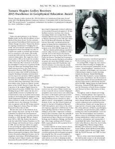
Figure 1. (left) Fixed radiative cooling profile and (right) relaxation inverse time constant used in each model. Thin lines in each plot represent the zero axis and approximate tropopause. radiative transfer and surface flux schemes. In contrast, the CSRM is a three-dimensional representation of the atmosphere wherein convective processes are explicitly modeled at the prescribed resolution. [6] Although each model has the capability to modify the height-dependent radiative cooling rate over time, this feature is replaced in all models by a constant radiative cooling scheme. In this way, we avoid cloudradiative feedbacks and simplify the system of study. The radiative cooling profile (see Figure 1) is a constant Qrad 521:5 Kd21 from the surface to near 200 hPa and decreases linearly to zero near 100 hPa. In addition, temperature and moisture relaxation to the radiative convective-equilibrium (RCE) profile of a previous run is imposed in each model near and above the tropopause in order to prevent the models from obtaining nonphysical values in a region where adjustment due to convective activity is weak. The adjustment time constant, also shown in Figure 1, increases from zero near a height of 160 hPa to a constant value of 0:5day 21 at and above the tropopause (�100 hPa ).� All models use a constant sea surface temperature of 28 C. 2.1. System for Atmospheric Modeling [7] The CSRM used in this study is the System for Atmospheric Modeling (SAM) version 6.8.2. A previous version of this model was described in Khairoutdinov and Randall [2003]. In this study, we use 28 vertical levels extending to 32 km with 2 km horizontal resolution on a square 128 km domain. The vertical grid spacing is �100 m near the surface and coarsens to �1km in the midtroposphere, similar to what is used in the Superparameterized Community Atmosphere Model [Khairoutdinov and Randall, 2001]. A bulk formula is used for surface sensible and latent heat fluxes and a simple Smagorinsky-type closure is used for the effect of subgrid-scale turbulence. The surface wind speed and exchange coefficients are 5ms21 and 131023 , respec-
tively. Results with higher vertical resolution (64 vertical layers instead of 28) are broadly similar [see, e.g., Kuang, 2012]. 2.2. MIT Single-Column Model [8] The Massachusetts Institute of Technology (MIT) Single-Column Model (MSCM) is a one-dimensional model and is somewhat modified from that used in � ´ -Rothman [1999]. The convective Emanuel and Zivkovic parameterization used is the CONVECT subroutine. See Emanuel [1991] for extensive theoretical background and a detailed description of CONVECT. The scheme takes as input columns of absolute temperature, specific humidity, winds, and pressure. In turn, CONVECT predicts tendency columns of temperature, moisture, and momentum. In the simplified form used in this paper, the single column model is essentially a wrapping function for the convective parameterization, although it also calculates turbulent fluxes at the surface and radiative cooling aloft, effects not present in the convection scheme. [9] The convection scheme represents shallow and deep convecting, precipitating cumuli and contains a dry adiabatic adjustment. Sea surface temperature and surface winds are held constant. Although MSCM incorporates convective downdraft feedback in the aerodynamic flux formulae, we disabled this feature to match the other models in the study. We also disable the Reynolds-type correction terms in the flux formulae � ´ -Rothman (see equation (6) in Emanuel and Zivkovic [1999]) for the same reason. Interactive radiation is shut off, which also disables the interactive cloud scheme. Parameter values used for MSCM are shown in Table 1. Although we employ many of the convective scheme � ´parameter values reported in Emanuel and Zivkovic Rothman [1999] some internal parameters have been modified in subsequent tunings by the model author. This column model, as well as the one described below,
511
HERMAN AND KUANG: RESPONSE FUNCTIONS OF PARAMETERIZATIONS Table 1. Parameters Used in MIT Single-Column Modela
Table 2. Parameters Used in Diabat3a
Parameters Used in MSCM
External Parameters Used in D3
Time step (min) Interactive radiation Interactive surface temperature Interactive water vapor Dry adiabatic adjustment Moist convection Surface wind speed (m s21) Cubic profile of omega Apply WTG approximation Surface drag coefficient Sea surface temperature (� C) Autoconversion threshold, �lcritical (g g21) Critical temperature, Tlcritical (� C) Mixing parameter, K (mb21) Fractional area of unsaturated downdraft, rd Fraction of precipitation falling outside cloud, rs Pressure fall speed of rain (Pa s21) Pressure fall speed of snow (Pa s21) Evaporation coefficient for rain Evaporation coefficient for snow Convection buoyancy threshold (K) Relaxation coefficient, a (kg m22 s21 K21) Relaxation coefficient, DAMP
Value 5.0 n n y y y 4.8 n n 1.0 3 1023 28.0 0.0011 255.0 0.03 0.05 0.12 50.0 5.5 0.9 0.6 0.9 0.015 0.05
Time step (min) Temperature relaxation rate Wind relaxation rate Mixing constant, kc (ks– 1) Stratiform rain constant, ks (ks21) Convective rain constant, kp (ks21) Evaporation rate constant, ke (ks21) Surface drag coefficient Terminal velocity of raindrops (m s21) Terminal velocity of snowflakes (m s21) Top of planetary boundary layer (km) a
Value 5.0 0.0 0.1 0.03 0.1 0.0006 300 1:031023 4.0 2.0 1.25
Only parameters considered relevant to this study are listed here.
prescribed constant rate. As in MSCM, the surface temperature and wind speed are held constant and aerodynamic flux formulae determine sources of latent and sensible heat from the surface. Parameter values for D3 were chosen to match those used in Raymond and Herman [2011]. The parameter values used are shown in Table 2.
a
External parameters not listed are not read by the model, since certain options have been turned off. Only internal parameters considered relevant to this study are listed here.
employs constant vertical resolution of Dz5250 m and columns of 80 grid cells giving domain heights of 20 km. 2.3. Diabat3 [10] The diabat3 (D3) toy cumulus parameterization originates from the scheme introduced in Raymond [1994], is a slightly modified version of that described in Raymond [2007], and is here incorporated into a 1-D single-column model as in a recent study by Raymond and Herman [2011]. Refer to the appendix of Raymond [2007] for a detailed description. The scheme predicts convective tendencies and surface fluxes based on columns of potential temperature, total cloud water mixing ratio and momentum. Total cloud water is here defined to be vapor and condensates minus precipitation. Both surface fluxes and column tendencies of equivalent potential temperature, total cloud water mixing ratio and momentum are returned to the calling model. Convective tendencies are determined as the weighted sum of sources due to shallow (within the prescribed boundary layer) and deep convective modes. The weighting factor for deep convection is determined by the amount of convective inhibition (CIN) above the subcloud layer. The sources returned by the scheme are calculated via a conservative adjustment toward a mass-weighted average within the convective layer, combined with a distribution of surface fluxes throughout the depth of the convective column according to a rate constant. Deep convective tendencies are furthermore a strong function of the saturation fraction. [11] In addition to the above effects, the moisture source is diminished by convective and stratiform precipitation and augmented by evaporation of precipitation. Each of these processes occurs at a unique,
3.
Methods of Analysis
[12] We employ two complimentary analysis techniques for intercomparison of the two column models and the CSRM. In this way, we determine the instantaneous convective responses to anomalous temperature and moisture states and the evolution of these states over an 18 h period for each model. These analyses are derived through two different methods, the construction of a representative matrix via an inverse problem, and the instantaneous perturbation of the forward model. 3.1. Matrix Inversion [13] We begin with the matrix inversion technique described in Kuang [2010] in which convective tendencies are determined using dx 5Mx; dt
ð1Þ
where x is a state vector of the respective model of the form � �T x5 T 0surf ; …; T 0top ; q0surf ; …; q0top
ð2Þ
representing stacked columns of temperature (T) anomalies from the surface to near 15 km and specific humidity (q) anomalies from the surface to near 12 km. The anomalies are with respect to a predetermined RCE state and the matrix M contains time rates of change effecting the linear transformation of x into dx=dt. [14] The matrix M is not known a priori and must be derived from the behavior of each model. Following the method outlined by Kuang [2010], we obtain the response matrix by inverting
512
HERMAN AND KUANG: RESPONSE FUNCTIONS OF PARAMETERIZATIONS
Figure 2. RCE columns of temperature for (left) SAM, (middle) the column models, and (right) relative humidity for all models. The dots at the right edge of the temperature plots indicate the vertical grid spacing for each model (D3 and MSCM have identical grids). The lines illustrating the relative humidity profile are broken near the tropopause due to supersaturation in the region. All relative humidity plots are rendered from internal values of RH or specific humidity and saturated specific humidity for each respective model. Y5MX; [15] where the columns of Y are tendencies of the form � � dxi dTi dTi dqi dqi T yi 5 5 ; …; ; ; …; dt dtsurf dttop dtsurf dttop
ð3Þ
and the columns of X are each of the form (2). The ith column of Y and the ith column of X are assumed to be uniquely related, so that xi gives rise to yi and vice versa. [16] We first obtain an RCE state for each model, letting it run until the prognostic variables reach statistical equilibrium. Time-averaged columns from the equilibrium state are then used to initialize the control and per-
turbation runs in each case. The RCE columns of temperature and relative humidity are shown in Figure 2. [17] Unique positive and negative perturbation tendency profiles are then applied to either T or q in separate runs for each vertical grid level. The tendencies are maintained until the model obtains a new RCE state under the additional forcing. The jth perturbation used in the CSRM, which takes the form of the sum of delta and Gaussian functions is defined as � � � pj 2pi �2 fj ðpi Þ5dij 1exp 2 ; 75 hPa
ð4Þ
where pi is the local pressure value, pj is the jth pressure value up from the lowest model level, and dij is a delta
Figure 3. Anomalous temperature profiles corresponding to applied temperature tendency perturbations near 730 and 850 hPa for all three models. The applied tendencies for SAM (dashed) and the column models (solid) are shown at far left. The zero axis is shown as a dashed line in each plot. Note that the vertical grid spacing differs between SAM and the column models, so that the applied tendencies occupy slightly different layers. 513
HERMAN AND KUANG: RESPONSE FUNCTIONS OF PARAMETERIZATIONS
Figure 4. Same as Figure 3 only with anomalous moisture profiles for applied temperature tendencies.
function at the jth model level. This form is not optimized and is chosen simply to include both a relatively broad perturbation and a perturbation over the scale of individual model layers. The form is identical to that used in Kuang [2012]. Only the delta function portion is used to perturb the column models as we find this gives the best accuracy and the closest match to results of the forward model approach (see Appendix B). The amplitudes of applied dT/dt and dq/dt are 0:5 Kd21 and 0:2 gkg 21 d21 for SAM, 1:0 Kd21 and 0:4 gkg 21 d21 for D3, and 0:25 Kd21 and 0:25 gkg 21 d21 for MSCM, respectively. These values were optimized for accuracy. The perturbation amplitude is reduced by half in SAM when the level defined by pj exists above 10 km. This is done in order to prevent the CSRM from obtaining nonphysical values of temperature and moisture where convective adjustment is minimal. In the column models, this attenuation had little effect on the results except to increase the linear dependence of the state matrix X and was not used. [18] We maintain the prescribed tendency forcing for periods of 10,000 days for SAM and 500 days for each
column model, which are sufficient intervals to capture the resulting statistical equilibrium in each respective case. Temporal averages of the final RCE states are obtained and results from the positive and negative perturbations are combined to form a centered difference approximation of the columns of X. Columns of anomalous temperature and moisture in equilibrium with applied tendencies in the form of (4) are shown in Figures 3–6. [19] Since the convective response must balance the prescribed forcing tendency in order to obtain the new equilibrium state, each yi is simply minus the prescribed tendency corresponding to each xi . The prescribed tendency in this case includes the stratospheric relaxation described in section 2 because the relaxation is imposed as part of this study, not by the original convective scheme. [20] To ensure accuracy over a range of stochastic variation, we calculate an ensemble of X and Y for each column model and average them together. To each ensemble member, we apply a unique set of random perturbations in T and q over the forcing period. These are
Figure 5. Same as Figure 3 only with anomalous moisture profiles for applied moisture tendencies. 514
HERMAN AND KUANG: RESPONSE FUNCTIONS OF PARAMETERIZATIONS
Figure 6. Same as Figure 3 only with anomalous temperature profiles for applied moisture tendencies.
described in detail in Appendix B. This treatment improves the linearity of each model response, but also eliminates the high-vertical-wave number response modes that persist over the forcing period, particularly in MSCM. These modes exist as small, grid-scale variations in T and q and contribute to linear dependence in X. Since they contribute negligibly to the larger-scale model behaviors of interest in this study, we eliminate them via ensemble averaging. Similar smoothing occurs in the CSRM, where internal stochastic noise over the long forcing interval takes the place of imposed random perturbations. 3.2. Forward Calculation [21] In order to verify the inverse results for the column models, we also use a forward approach with D3 and MSCM whereby we perturb each model with anomalies in the temperature and moisture fields and then observe the convective tendencies and state anomalies following the instant of perturbation. As in the above section, we let each model run to equilibrium and then apply a single perturbation in one of the state vectors at a single time step. The behaviors of T, q, dT/ dt, and dq/dt following these perturbations describe convective responses similar to those sought in section 3.1. In order to maintain consistency with Kuang [2010], the shape of the jth applied perturbation matches the perturbations used in that paper and takes the form " � �# pi 2p0 1ðj21=2Þ 2 xj ðpi Þ5exp 2 75 hPa
ð5Þ
for perturbations above the lowest model layer and � � � pi 2p0 �2 xj ðpi Þ5exp 2 30 hPa
ð6Þ
at the lowest model layer, where pi is the local pressure value and p0 is the surface pressure. We use perturba-
tion amplitudes in T and q of 0.5 K and 0:5gkg 21 , respectively. We performed the same comparison using amplitudes an order of magnitude smaller and obtained similar results, not reported here. [22] Since the forward calculation method involves scrutiny of the time-dependent state and tendency vectors following instantaneous perturbations, it is possible that the observed response depends on the unperturbed model state. To obtain a robust response from the forward calculation, we derive the average of an ensemble of 40 different model runs. Each ensemble member is perturbed at a unique time step in order to minimize effects due to the initial state. As described previously for the inverse experiment, random temperature and moisture perturbations are also applied at different locations within the column over the ensemble. These are described in Appendix B. Again, we combine the positive and negative results to obtain average linear perturbations, which we take to represent the convective responses to anomalies in T and q of the respective model. [23] One complication here is that the column models employ different assumptions about convective response time. For D3, this time is negligible, while for MSCM, the adjustment time is a function of parameters controlling the relaxation of the convective vertical mass flux to values implied by subcloud layer quasiequilibrium. Thus, for the purpose of comparison, we shut off the relaxation mechanism in MSCM, which eliminates the convective response time. [24] In order to make a parallel comparison across the models, we average the response tendencies over the 2 h immediately following the perturbation. We do this in order to diminish the influence of fast-decaying eigenmodes in the response matrix M––an issue of particular importance in SAM. Intercomparisons of anomalous tendency vectors derived from the forward model and inversion techniques show strong similarities (see Appendix B). We thus feel confident that evaluations can be made based on these experiments.
515
HERMAN AND KUANG: RESPONSE FUNCTIONS OF PARAMETERIZATIONS
4.
Results
4.1. RCE Columns of Temperature and Relative Humidity [25] Equilibrium columns of temperature and relative humidity are calculated from temporal averages of the RCE run for each model (see Figure 2). We attempted to set the cloud base to the same pressure level for all three models in order to define a consistent boundary by which to differentiate above and below cloud base properties across the set of models. To force the respective column model RCE cloud base levels to match that of SAM, a parameter was set in D3 to define the top of the boundary layer in that model. The effect of this setting is to create kinks in the temperature and humidity columns (see Figure 2) near 900 hPa. These kinks are due to the different modes of convective adjustment occurring in D3 above and below the top of the boundary layer (see section 2.3). A cloud base-like layer then occurs near 930 hPa as evinced by the gradient in relative humidity below that level. The cloud base level is determined dynamically in MSCM, so we simply use the RCE profile of D3 to initialize MSCM. Each column model undergoes some adjustment before attaining its respective RCE state under the imposed forcing, which leads to divergent thermodynamic profiles. [26] While the temperature profiles in the column models are similar to that of SAM, the relative humidity profiles of all three models differ significantly. A rigorous matching of the columns through parameter selection would likely take each model far outside the realm of its author’s intention and was not used. However, it is interesting that the models arrive at such different profiles given the same initial thermodynamic state. Part of the difference comes from the behavior of MSCM, which immediately rains out much of the column moisture after initialization. This suggests MSCM interprets the stability or the precipitation efficiency of the initial state quite differently from the other models. 4.2. Steady State Responses to Temperature and Moisture Tendencies [27] The initial step in forming M in the matrix inversion approach is to apply tendencies in T and q to the RCE state of each model until a new equilibrium state occurs. A comparison of the models under a few forcing cases lends some insight into model characteristics. In this section, we use identical forcing functions and amplitudes in order to minimize differences due to the method of analysis. [28] The changes in temperature due to warming tendencies near 730 and 850 hPa are shown in Figure 3. The response in SAM is to shift the temperature profile by approximately the difference between two moist adiabats, with slightly more warming occurring near the forcing layer. MSCM has a similar response, except the 850 hPa case shows a cool layer immediately above the forcing layer. In contrast, D3 warms only the forcing layer itself and the boundary layer. [29] Changes in specific humidity due to the same warming tendencies are shown in Figure 4 and illustrate
similar, respective response characteristics. As the atmosphere warms in SAM, the saturation vapor pressure increases and thus more vapor can exist at each pressure level in the column, assuming relative humidity stays about the same. The change in specific humidity is greater at lower levels where the specific humidity is greater. This response was identified in Kuang [2010] as the least damped eigenmode of the resulting M matrix for SAM. Again, MSCM shows some of this behavior, though strong moistening and drying occur at and above the forcing layer, respectively. The response is more localized in D3, where moistening only occurs at the forcing layer and in the boundary layer. [30] Adding moisture leads to a similar pattern in column moistening for each respective model (see Figure 5), though drying above the forcing layers in MSCM is here replaced by layers of weaker moistening. Interestingly, while changes in absolute temperature (see Figure 6) for SAM and MSCM again seem to be shifts of moist adiabats, MSCM doesn’t exhibit any cooling above the forcing layer when moistening is applied, unlike for the applied warming case. Also, D3 shows significant upper tropospheric warming not evident when warm tendencies are applied. Again, D3 is missing the moist adiabat shift seen in the other models. See Appendix A for a more detailed comparison of the tendency forcing. 4.3. Convective Tendency Responses to Temperature Anomalies [31] The linear response function analysis described by Kuang [2010] provides a parallel format to compare the convective responses of differing atmospheric models. In this study, we attempt a more robust comparison by averaging the response tendencies over the first 2 h. This is to minimize the effects of the fastest-decaying eigenmodes, which dominate the instantaneous response functions yet have little influence upon the longer time scale behavior of the state vectors. Since the matrix M is derived from the inverse of X, discrepancies in X will cause the most significant errors to occur in the fastest decaying eigenmodes since jdkj / jk2 jjjdXjj, where jjdXjj is a matrix norm of the errors in X (the matrix Y is prescribed and thus contributes no error). The responses are obtained from a time-averaged modification of (1) h dx x0 5MxðtÞ5 expðM2hr Þ2I� dt 2hr
ð7Þ
where M is derived from the inverse technique described in section 3.1 and I is the identity matrix. [32] The response functions are shown in Figures 7 and 8. Conspicuous kinks in the responses for D3 and MSCM are correlated with steep relative humidity gradients near 600 hPa in each column model (see Figure 2). This artifact highlights the significance of the relative humidity profile in the model response. [33] We begin a detailed analysis by examining the 2 h average response to a near-surface temperature anomaly in each models (top row, Figure 7). As the responses
516
HERMAN AND KUANG: RESPONSE FUNCTIONS OF PARAMETERIZATIONS
Figure 7. Time-averaged (2 h) anomalous convective heating (circles) and moistening (crosses) profiles associated with warm anomalies applied at different levels. The shape of each 1 K warm anomaly is shown at far left in each row. Horizontal axes for each model are constant throughout to facilitate comparison.
517
HERMAN AND KUANG: RESPONSE FUNCTIONS OF PARAMETERIZATIONS
Figure 8. Same as Figure 7 except for applied moist anomalies. Peak values of the temperature tendency in D3 for the 500 and 350 hPa cases are 9:8 and 13:7 Kd21 , respectively. are approximately linear, only warm and moist (not cool or dry) anomalies will be considered in the analysis of temperature and moisture, respectively. Warm
anomalies near the surface elicit cooling in the subcloud layer in all models. SAM and MSCM show warming directly above the anomaly, indicating adjustment
518
HERMAN AND KUANG: RESPONSE FUNCTIONS OF PARAMETERIZATIONS
within the subcloud layer, and moistening and drying in the upper and lower part of the subcloud layer, respectively. D3, however, seems to be missing this overturning mechanism. Aloft, there is minimal response in SAM and D3, while significant warming and some drying occur in MSCM. [34] For warm anomalies applied to the modeled free troposphere, SAM responds with deep tropospheric cooling extending upward from the perturbed layer and a smaller localized moistening region at or just below it, both of which decrease in amplitude monotonically with the height of the perturbed layer. In addition, SAM warms just below the perturbed layer and warms and moistens the subcloud layer in these cases. The magnitudes of the column model responses are not monotonic with the height of the perturbed layer and cooling is mostly local, near the layer of the imposed warm anomaly. While D3 shows a cooling maximum collocated with the perturbed layer in each case, MSCM cools just above and warms just below each perturbed layer. This is an interesting feature that effects behavior similar to SAM, as explained later in section 4.5. [35] The warming below the anomalous layer in SAM is likely due to compensating subsidence outside convective updrafts, an explicitly modeled effect in the CSRM. In MSCM, compensating subsidence is expressed in terms of the convective mass flux and the entrainment and detrainment rates throughout the convective column. The cooling seen in D3 is largely due to evaporation of precipitation formed aloft, as suggested by the simultaneous moistening at the anomalous layer, but is also due to the relaxation of local he to its mean value in the convective column. [36] Neither column model shows warming of the subcloud layer, though this response of the CSRM makes intuitive sense: when deep convection is reduced, surface fluxes should increase the low-level entropy. In this way, there seems to be a lack of communication between the free troposphere and the subcloud layer in the column models. The broad layers of slight warming shown below the perturbed layer in D3 and MSCM for the 500 hPa case are not seen in SAM. The warming in D3 is likely due to the conservative relaxation of he ; though in MSCM, it indicates the onset of a broad warm layer beneath the imposed anomaly seen in both SAM and MSCM after 6 h (see Figure 9). Note that, while SAM strongly cools the upper troposphere in each case, D3 only cools the upper troposphere for the 800 hPa case, and does so at a slower rate. In contrast, MSCM exhibits almost none of the cooling one expects after imposing a significant inversion in the free troposphere. [37] More significant differences between SAM and the column models are evident in the convective responses of moisture to applied warm anomalies in the free troposphere. While the moistening that occurs just below the warm anomaly in the CSRM is likely due to the detrainment and storage of moisture below an inversion layer, D3 places the moistening layer precisely at the anomaly and furthermore shows stronger mois-
tening tendencies for higher level warm anomalies. As mentioned above, the moistening in this case is most likely due to evaporation of precipitation from deep convection. The evaporation component in D3 is disrupted for the 350 hPa perturbation, however, due to a strong relative humidity gradient leading to supersaturation above 360 hPa (see Figure 2); in the saturated region, evaporation cannot occur. [38] Like D3, MSCM exhibits somewhat complementary moistening and heating responses; for example, a midtropospheric (650 hPa) warm anomaly is met with weak moistening above and drying just below it. But unlike SAM or D3, MSCM shows a deep drying layer beneath each respective warm anomaly for the 800–500 hPa cases. And just as the column models lack subcloud layer warming responses, they show less moistening in this layer than SAM. [39] Finally, the significant warming and drying above 300 hPa for the 800 and 650 hPa temperature perturbations in D3 is unmatched by either SAM or MSCM, and is correlated the supersaturation above 300 hPa in that model. This suggests that the saturation value causes nonphysical processes to occur in this layer. 4.4. Convective Tendency Responses to Moisture Anomalies [40] We now describe responses to moisture anomalies in each model, illustrated in Figure 8. Convective responses to subcloud layer moisture anomalies suggest strong agreement in that all models treat a low-level moist anomaly with drying in the subcloud layer and warming aloft. While SAM also shows a moistening and drying response in and above the subcloud layer, D3 shows only the drying above and MSCM only the moistening. Also, MSCM uniquely shows drying near 650 hPa. [41] Free-tropospheric moist anomalies in SAM are met with localized drying at the anomalous layer and in the subcloud layer. The column models also dry near the anomalous layer, but show little evidence of subcloud layer drying. An exception is the 800 hPa case, where D3 shows significant subcloud layer drying, although MSCM moistens the layer in this case. If we take SAM’s consistent subcloud layer drying to indicate the ventilation of low levels by enhanced deep convection, D3 and MSCM are missing this well-documented feature [Masunaga, 2012]. Also, the localized drying in MSCM is insignificant and somewhat offset from the anomalous layer compared to that of SAM and D3. In addition to the local drying response, SAM moistens below the anomalous layer for upper-elevation moist anomalies. This response is evident in D3, but is missing from MSCM. [42] A stronger contrast between SAM and the column models is evident in the free tropospheric temperature response. SAM shows top-heavy warming at and above the anomalous layer. Also, SAM shows cooling just below the anomalous layer and close to the surface. MSCM and D3 give highly localized warming at the anomalous layer and none above it. This warming
519
HERMAN AND KUANG: RESPONSE FUNCTIONS OF PARAMETERIZATIONS
Figure 9. Decay of anomalous temperature state vectors following applied temperature anomalies at five different pressure layers occurring at t 5 0. Anomalous temperature perturbations are shown at left in each row. Other columns represent magnitude of state vector after t 5 2 h, t 5 6 h, t 5 12 h, and t 5 18 h, respectively. State vectors for SAM (black), D3 (red), and MSCM (blue) are shown.
520
HERMAN AND KUANG: RESPONSE FUNCTIONS OF PARAMETERIZATIONS Table 3. Response Differences Between D3 and SAMa Location of Applied Anomaly
T Following WA
q Following WA
Subcloud layer
No SCL warming
Negligible SCL drying; no moistening above SCL
Above cloud base (800 hpa) Middle troposphere (650–350 hpa)
Minimal early cooling aloft� ; no later warming aloft� No early cooling aloft� ; no later warming aloft�
Moistening at WA, not below it� ; prolonged SCL moistening� Moistening at WA, not below it� ; minimal SCL moistening�
Upper troposphere (350 hpa)
Slow reduction of WA� ; no warming below WA
Moistening at WA, not below it� ; no later moistening below WA�
T Following MA
No SCL cooling� ; strong warming at ma; cooling (not warming) aloft Strong warming at MA; negligible warming aloft; low elevation cooling too early Strong warming at MA; low elevation cooling too early;
q Following MA MA persists for much longer; dry layer above SCL persists for much longer; DT=Dq � 5=2 MA persists for much longer� ; DT=Dq � 5=2 No early SCL drying� ; DT=Dq � 5=2 MA reduced very quickly; no early SCL drying� ; no low-tropospheric drying� ; DT=Dq � 5=2
a Differences are stated in terms of how D3 differs from SAM and are summarized in terms of temperature and moisture changes associated with warm (WA) and moist anomalies (MA). An asterisk (� ) indicates the characteristic is shared between D3 and MSCM and SCL indicates the subcloud layer.
response is negligible in MSCM except for the 500 and 350 hPa cases, indicating that the added latent heat is not used to warm the column for the lower elevation cases. The highly complimentary warming and drying responses in D3 suggest this model is primarily concerned with condensing the moist anomaly and latent heating, rather than modifying the extant convective state. In the case of strict condensation, moist static energy is �conserved and we expect a ratio of jDTj=jDqj5 Lv =Cp 31023 � 2:5. Since D3 maintains a ratio of � 2:4 for all free tropospheric cases, this model exhibits localized condensation almost perfectly. Ratios of dT/dt to dq/dt for the 800–350 hPa cases are 0.5, 0.5, 1.1, 1.7 for SAM; 2.4, 2.4, 2.4, 2.3 for D3; and 0.3, 0.3, 1.3, 1.2 for MSCM, respectively. [43] Like SAM, MSCM exhibits ratios of warming to drying at the anomalous layer that increase with height––though this behavior is not strictly monotonic for MSCM. This reflects the diminishing saturation specific humidity for higher elevation perturbations. In SAM, rising parcels moistened by the imposed anomaly have a shorter path to their respective levels of stability; this foreshortens the layer of moistening above the imposed anomaly, which in turn increases the likelihood of local saturation. A conspicuous side effect of conservative adjustment is illustrated in the response for the 800–500 hPa cases, where D3 shows cooling and moistening above the perturbed layer. [44] As mentioned, SAM appears to consistently advect the added moisture aloft, where it is used to warm the column. The local drying in this model is thus partly due to moisture divergence out of the layer rather than just to local condensation. These indications suggest that a significant moist anomaly should lead to significant changes in the thermodynamic state above the anomaly, though there is little evidence of this in MSCM or D3. [45] Below the anomalous layer in SAM and D3, inflection points exist in the temperature and moisture tendencies for the 650–350 hPa cases. These cause
downward broadening of the initial moisture anomaly and also an inflection point in the resulting temperature anomaly. These features are not evident in MSCM. Differences in convective response functions between SAM and the column models are summarized in Tables 3 and 4. 4.5. Evolution of State Vectors Following Warm Anomalies [46] The response tendencies discussed in sections 4.3 and 4.4 emphasize the fast-decaying eigenmodes of each system, particularly those acting over the first 2 h following applied perturbations. To observe the changes due to all the modes at the time scale of interest, it is necessary to examine the evolution of the state vectors T ðz; tÞ and qðz; tÞ over the time period following applied perturbations. Thus, we choose a period of 18 h following applied anomalous states; the end of this period places more emphasis on eigenmodes with smaller decay rates. [47] State vector growth and decay is illustrated in Figures 9–12 for all models. The state vector anomalies for each model are derived from M and are calculated using xj ðtÞ5x0j expðMtÞ;
ð8Þ
where xj ðtÞ is the time-dependent state vector corresponding to the jth anomalous state, x0j , at time t. The imposed anomalous states take the form of (5) and (6) and the times of interest are: 2 h past the occurrence of the anomalous state (in order to capture the net effect of the tendencies described in sections 4.3 and 4.4); 6; 12; and 18 h. [48] One characteristic that appears to be a manifestation of the height-dependent nature of the convective quasiequilibrium response discussed by Tulich and Mapes [2010], Kuang [2010], and Raymond and Herman [2011] is the nearly monotonic decrease with height in the decay of the imposed temperature anomaly shown
521
HERMAN AND KUANG: RESPONSE FUNCTIONS OF PARAMETERIZATIONS Table 4. Response Differences Between MSCM and SAMa Location of Applied Anomaly
T Following WA
q Following WA
T Following MA
Subcloud layer
Warming aloft
Above cloud base (800 hpa)
Minimal early cooling Moistening at WA, not No SCL cooling� ; late aloft� ; later warming below it� ; prolonged SCL warming aloft aloft only in shallow moistening� layer� No warming aloft� ; Less early cooling aloft� ; no Moistening at WA, not warming below WA; no below it� ; minimal SCL no cooling below MA later warming aloft� moistening� ; drying below WA Minimal warming at MA Slow reduction of WA� Negligible moistening at WA; no later moistening � below WA ; drying below WA
Middle troposphere (650–350 hpa) Upper troposphere (350 hpa)
Drying above SCL
q Following MA No drying above SCL; drying at mid troposphere MA persists for much longer� ; no early SCL drying MA persists for much longer; no early SCL drying� ; no moistening below MA MA persists for much longer; no early SCL drying� ; no lowtropospheric drying�
a
Same as for Table 3 but for MSCM.
in Figure 9. In contrast, however, while SAM expresses this height dependence at the 2 and 6 h times, the column models illustrate this preference for stronger decay at low levels at the 12 and 18 h times. Also, SAM nearly eradicates these anomalies at all levels after 18 h, but the column models do not. Such discrepancies in the treatment of anomalies on the diurnal time scale may be important for the ability of these models to express convectively coupled waves, as illustrated in Kuang [2010]. [49] Notably, all models agree that a near-surface warm anomaly is diminished after about 18 h. As predicted by the tendency shown in Figure 7, however, MSCM shows some temperature adjustment aloft over this interval. The decay of a warm anomaly above the subcloud layer gives a more mixed response across the models. The response functions for an anomalous warm layer at 800 hPa suggest that all models will elicit some cooling in the column above the anomalous layer, though the time dependence of this response varies significantly across the models. SAM has cooled the troposphere above the anomaly and warmed the subcloud layer by �0:2 K after 2 h. This suggests that deep convective heating has been significantly attenuated over this interval. Thereafter, SAM weakens the original anomaly, cools the subcloud layer and warms the upper troposphere until there exists a warm anomaly uniform in height through the depth of the troposphere after 18 h. [50] In contrast, after 2 h, the column models have neither cooled the upper troposphere nor warmed the subcloud layer. By 18 h, D3 has approximated the uniform warm anomaly up to �750 hPa , but has only cooled the upper troposphere. MSCM never warms the subcloud layer, and shows a layer of cooling aloft after 6 h. SAM likely warms the upper troposphere via the release of instability below the anomaly, leading to invigorated deep convection. This process seems to occur somewhat in MSCM, though the warmed layer aloft is considerably shallower than that in SAM; the process appears to be missing entirely from D3. Perhaps in retaining the original warm anomaly for a longer pe-
riod, the column models maintain a strong stable layer and thus stifle deep convection well beyond the release of SAM’s instability. If this is the case, the column models seem to lack mechanisms to deplete the stable layer. SAM does this by rapidly reducing the original anomaly while simultaneously warming the subcloud layer. The latter effect never occurs in MSCM and only occurs in D3 after �12h. Since each model uses the same surface flux forcing in this experiment, it may be the way that each model incorporates those fluxes into the convective response that makes a difference here. The warming aloft after 12 h in SAM is an example of cyclic response activity that manifests as complex eigenvalues of the response matrix M. Since unstable modes are not possible in M, the upper elevation warming must subside at a later time (not shown). [51] A similar pattern occurs for the 650 hPa case. SAM responds with even stronger cooling aloft, with a warm subcloud layer, followed by a uniform warm layer from the surface up to the original anomaly. The low-elevation warming is then quickly followed by warming aloft. Again, the column models retain the original anomaly throughout the entire period of study and show negligible warming below it. As the response function shown in Figure 7 predicts, MSCM does show some cooling aloft, but not as deep or as significant as that which occurs in SAM. Also, while peak cooling aloft occurs in SAM over 2–6 h, the peak in MSCM occurs during the 12–18 h interval. [52] As in the 800 hPa case, SAM’s response begins to assume the form of a shift of a moist adiabat after 18 h. Again, the stable layer near the original anomaly is decreased rapidly in SAM by the joint action of the contracting anomaly itself and by the warm layer below it. Neither effect occurs to a significant degree in the column models, so that stability is maintained throughout the 18 h period. As predicted by the inflection point shown in the response function, MSCM acts to push the warm anomaly downward. Although this acts to warm the lower troposphere, it neither minimizes the anomaly, nor broadens it in the vertical, so that stability cannot be reduced by this mechanism alone.
522
HERMAN AND KUANG: RESPONSE FUNCTIONS OF PARAMETERIZATIONS
Figure 10. Same as Figure 9, except for time-dependent moisture vectors following applied temperature anomalies. Note that the horizontal scales of the lower three rows are 40% smaller than those of the top rows. [53] Following the 500 hPa anomaly, SAM again cools aloft and warms below, quickly reducing the original warm anomaly. This is again followed by warming
aloft and presumably an approach to a uniform warm anomaly after the 18 h period. The 350 hPa response is similar, except no cooling is seen aloft. In these cases,
523
HERMAN AND KUANG: RESPONSE FUNCTIONS OF PARAMETERIZATIONS
the column models neither cool aloft, nor significantly reduce the original anomaly. However, MSCM does warm below the anomalies and moves them to lower elevations. This shift is too rapid to be explained by parameterized downdrafts in MSCM, which we have measured to be at most on the order of 1=2 hPa h21 . Though, levels of entrainment into and detrainment out of the cloud drafts undergo large changes in MSCM (not shown) near the anomaly after it is imposed. [54] Less concordance is illustrated in the evolution of moisture state vectors following applied temperature anomalies (see Figure 10) We have already noted the lack of drying response in D3 following the warm anomaly imposed at 1000 hPa. There is negligible change in low elevation moisture for this model throughout the period of study in this case, while SAM and MSCM dry the subcloud layer and moisten just above it. This suggests D3 is missing a mechanism to parameterize the subcloud layer overturning that occurs for a surface-layer instability. This makes sense, since much of the adjustment in D3 is largely uniform over the depth of the subcloud layer. [55] The column model responses to perturbations at 800 hPa qualitatively mimic that of SAM, though over a different time scale. All three models generate a moist anomaly in the subcloud layer after 2 h. At later times, moisture appears near the level of the original warm anomaly. However, SAM places this moist layer just below the original anomaly and it reaches maximum amplitude at �6h. The column models show a moist layer collocated with the original anomaly, but they continue to increase through 18 h. The time evolution of moisture in the subcloud layer also differs from that of SAM. The dry layer that forms above the imposed warm anomaly in SAM after 6 h also occurs in MSCM, though higher up in the troposphere. This effect is negligible in D3, however. An interesting feature is the matching moist anomalies at 800 hPa in D3 and MSCM. It makes sense that D3 forms a moist anomaly over a warm layer, due to this model’s proclivity to local phase changes; however, MSCM has already moved its warm anomaly down to 850 hPa by 18 h. This suggests that the adjustment mechanism here is a slow response to the original warm anomaly, rather than an immediate effect due to the extant temperature state. [56] Responses to the 650 hPa perturbation are more varied. SAM and D3 show somewhat similar behavior for this case, but MSCM shows a broad layer of drying beneath the original warm anomaly. Also, the moist peak near 650 hPa in MSCM is much larger than in either D3 or SAM and again is offset in height from the corresponding temperature anomaly after 18 h. Interestingly, D3 is also missing the midlevel moistening response. In SAM, this appears to be a downward broadening of moisture that has collected beneath the imposed temperature anomaly after 2 h. If this process is due to low-level convection and mixing, it may not occur in D3 if the model’s bimodal structure doesn’t allow convective adjustment to occur only in the lower half of the deep convecting column. Differentiating
characteristics seen in the 650 hPa case are mostly repeated for the 500 and 350 hPa cases and will not be analyzed here. 4.6. Evolution of State Vectors Following Moist Anomalies [57] In a qualitative sense, the most robust behaviors across the set of models are the time-dependent moisture responses to applied moist anomalies (Figure 11), though some important differences do exist. Following the 1000 hPa moist anomaly, SAM quickly reduces the anomaly to 25% of its original amplitude and dries the upper subcloud layer by 2 h. The original moist anomaly is reduced almost completely after 18 h, while slight moistening occurs aloft. MSCM reduces the anomaly at nearly the same rate as SAM, though, as predicted by the tendencies in Figure 8, there is some drying near 650 hPa. MSCM doesn’t dry the upper subcloud layer, but D3 models this response in tandem with SAM at 2 h; however, D3 retains the dry layer, as well as the original moist anomaly for much longer than the other models. [58] Each model responds to a moist anomaly imposed at 800 hPa in a similar way. SAM moistens the subcloud layer while reducing the original anomaly over the interval of study. By 2 h, SAM has already recovered from the subcloud layer drying that occurred early on (see Figure 8) and proceeds to moisten the subcloud layer over the remaining 18 h period. MSCM and D3 show similar behavior except over a longer time scale. In particular, the column models are slower to reduce the original anomaly and also to moisten the subcloud layer. The moistening is likely due to evaporation of precipitation or advection of the moisture anomaly via convective downdrafts. The latter is not possible in D3, however, since no downdrafts are parameterized in that model. [59] Following moist anomalies at 650 and 500 hPa, SAM depletes the anomaly to �40% over the period of study, while moistening the free troposphere below. The subcloud layer again moistens over this period from the initial drying that occurs within the first 2 h. In these cases, D3 matches the rate of drying of the original anomaly and even shows some of the lower-level moistening seen in SAM. D3 also shows some ventilation of the subcloud layer for the 500 hPa case at 6 h, which is much later than SAM’s analogous response occurring before 2 h. In contrast, MSCM retains much of the magnitude of the original anomaly, yet lowers its elevation by 10–30 hPa over the period of study. In addition, MSCM shows no moistening of the free troposphere below the anomaly and even shows slight drying just below the 500 hPa anomaly. [60] The highest elevation case is similar to those just described, except that SAM dries the lower troposphere toward the end of the period. This may be due to the increased moisture storage capacity of the upper troposphere (see analysis of temperature response, below), coupled with moisture advection from below via deep convection. SAM also shows moistening below the original anomaly down to 700 hPa, suggesting evaporation of precipitation. In this case, D3 reduces the original
524
HERMAN AND KUANG: RESPONSE FUNCTIONS OF PARAMETERIZATIONS
Figure 11. Same as Figure 9, except for time-dependent moisture vectors following applied moisture anomalies. Note the horizontal scale of the top row is half that of the other rows. anomaly significantly faster than SAM, while MSCM again retains and lowers it. Both column models dry the subcloud layer toward the end of the period, yet they
both miss the drying in the lower free tropospheric seen in SAM after 6 h. The column model response suggests evaporation of the precipitation formed at the
525
HERMAN AND KUANG: RESPONSE FUNCTIONS OF PARAMETERIZATIONS
Figure 12. anomalies.
Same as Figure 9, except for time-dependent temperature vectors following applied moisture
anomalous layer throughout the lower free troposphere; though, the shallow drier layer below the anomaly in MSCM at 18 h is puzzling.
[61] Some insight into the behavior of moisture states following applied moisture anomalies comes with examination of the corresponding temperature states shown
526
HERMAN AND KUANG: RESPONSE FUNCTIONS OF PARAMETERIZATIONS
in Figure 12. As indicated in Figure 8, all models warm the upper troposphere following the moist anomaly at 1000 hPa. This makes sense, since the added moisture should fuel deep convective heating aloft. The only significant difference in responses is in the extra warming in MSCM near 600 hPa. This may be due to condensation occurring there, as suggested by the decreased moisture at midtroposphere. [62] A stark contrast in the utilization of excess moisture across the set of models appears in the temperature response to the 800 hPa moist anomaly. Recall that SAM depletes the moist anomaly very quickly, while the column models retain much of the anomaly throughout the period of study. As we might expect, SAM warms the entire depth of the troposphere above 800 hPa. This is similar to the response following the 1000 hPa case, though the amplitude of warming is greater owing to the deeper anomalous moist layer. The warming again looks similar to the difference of two moist adiabats. Interestingly, MSCM also warms much of the troposphere, though beginning later than SAM. This is consistent with the result of the steady state forcing shown in Figure 6. Since MSCM depletes the moist anomaly more slowly, it makes sense that it warms the troposphere more slowly. What is surprising, considering the noted similarity in the evolution of column model moisture states, is the difference in the temperature states between the column models. D3 condenses all of its moisture right at the anomalous layer and shows no upper-tropospheric warming at all. In fact, the latent heating at the anomalous layer even acts to increase CIN, which stifles deep convection leading to a slight increase in radiative cooling aloft. This response is well predicted by the ratio of temperature to moisture tendencies shown in Figure 8. [63] SAM’s responses to the 650 and 500 hPa moist anomalies are similar to that of the 800 hPa case except there is some cooling below the anomaly, perhaps due to the evaporation of precipitation. Again, D3 shows strong warming at the anomalous layer, where most of the added moisture condenses, and negligible warming aloft. Since CIN is calculated from a weighted average over the lower levels of the modeled atmosphere, deep convection and thus upper tropospheric warming is more likely in D3 for higher elevation perturbations. D3 matches SAM’s rate of subcloud layer cooling for the 650 hPa case and shows strong cooling at 2 h below the anomaly for the 500 hPa case. The response shown for MSCM is puzzling, since this model shows very little warming at the anomalous layer for the 350 hPa case and none aloft for any case above 800 hPa. [64] We have seen that D3 consistently warms the anomalous moist layers, and a careful comparison with SAM for the 650 and 500 hPa cases is instructive. SAM and D3 reduce the moist anomaly at about the same rate such that, by 18 h they each retain about 40% of the imposed moist anomaly. However, while� SAM warms� the respective anomalous layers by �0:2 C and �0:35 C, respectively, D3 warms the same layers by � � �0:9 C and �1:3 C (see Figure 11). As mentioned above, the reason for this difference is suggested by
SAM’s deep warming response in these cases: advection of excess moisture aloft leads to warming aloft and less warming at the anomalous layer. Note that, even though SAM and D3 have similar relative humidity values at these layers before the anomalies are imposed, there is still a significant difference in how much moisture is condensed in place between these models. For moist anomalies near the tropopause where advection to higher elevations is not possible, even SAM responds with strong warming at the anomalous layer, again suggesting that the difference in behavior arises due to deficient moisture advection in D3. [65] Interestingly, MSCM provides nearly the same amplitude warming response as SAM at the anomalous layer for the 650 and 500 hPa cases, but like D3, doesn’t manifest any warming above the imposed anomaly. Since MSCM seems to condense just enough moisture to suitably warm the anomalous layer without advecting moisture aloft, like D3, this model seems deficient in advection in these cases. Unlike SAM and D3, MSCM retains most of the imposed moisture anomaly (see Figure 11) for these cases, which may be due to the reduced relative humidity values in this model at middle and upper troposphere. This notion is strengthened by the fact that, for the 800 hPa moist anomaly where the relative humidity profiles are more in agreement, MSCM depletes as much of the original moisture anomaly as D3. Even though part of the lack of warming aloft may be explained by the relative humidity profile in MSCM, there remains no evidence of warming aloft in any of the cases above 800 hPa, even as the rate of reduction of the moist anomaly is about half that of SAM’s, which is true for the 800 hPa case where warming does occur aloft. So, it seems that MSCM is missing this warming aloft ability only for moist anomalies above 800 hPa. [66] All models cool the lower troposphere to some extent following the moist anomaly at 350 hPa, though at different rates. As in the lower elevation cases, D3 warms the anomalous layer throughout the period of study. SAM also does this, but broadens the warm layer above and below the original anomaly, which suggests mixing into the nearby layers. MSCM also broadens the warm layer, while lowering its peak from 350 to 400 hPa over the period.
5.
Conclusions
[67] The goal of this paper has been to compare the convective response characteristics of two singlecolumn atmospheric models and also to compare them to a CSRM. We have shown that: (1) the forward model and inverse techniques described here allow comparison of differing atmospheric models (see Appendix B); (2) the resulting comparison indicates that the models of interest in this study exhibit distinct convective responses to temperature and moisture anomalies. [68] We used two complementary techniques to derive the convective response functions of the models, as well as to provide a form of cross validation of the results. The inverse matrix technique, which is best suited to a
527
HERMAN AND KUANG: RESPONSE FUNCTIONS OF PARAMETERIZATIONS
model that has finite convective response time, or convective memory, involves the construction of a linear transformation matrix that approximates the convective response of the model to an anomalous thermodynamic state. We expect errors in the transformation matrix to reduce accuracy early in the convective response due to the lower accuracy of the fastest-decaying modes in the matrix. The forward model technique illustrates convective response features in models that employ negligible convective response time. We expect the forward model to be sensitive to initial conditions, such that errors, i.e., response features that differ from the ensemble mean, occur later in the convective response. We have used both techniques in our analysis of the column models (see Appendix B). Since the results are similar, we conclude that our analysis is accurate, and represents typical model behaviors. We thus propose that the divergent states revealed by these techniques suggest a set of response behaviors at odds with the CSRM and perhaps the real atmosphere. 5.1. Responses to Temperature and Moisture Anomalies [69] The column models differ from the CSRM in several key aspects of convective response. For instance, a free-tropospheric stable layer appears to have an immediate effect on the rate of deep convection in SAM, such that significant cooling occurs aloft in a deep layer within 2 h of the imposed anomaly. Yet the column models show delayed cooling aloft for low-elevation anomalies and no cooling aloft for upper-elevation anomalies. Also, MSCM lacks subcloud layer warming in the case of a low-elevation warm anomaly. Following the cooling aloft in the case of anomalous stable layers, SAM warms a deep layer aloft that likely results from the release of instability below the stable layer. The column models do not seem to emulate the release of instability. Although MSCM does show cooling above warm anomalies at 800 and 650 hPa, it occurs much later than in SAM, and over shallower atmospheric layers. [70] Since a near surface warm anomaly causes neither drying in the lower, nor moistening in the upper subcloud layer, D3 may be missing a mechanism for subcloud layer overturning in the case of a surface instability. Unlike SAM, the column models do not moisten the free troposphere beneath warm anomalies placed above 800 hPa. MSCM takes this further and significantly dries this region, particularly at later times for the 650 and 500 hPa cases. [71] The lack of upper tropospheric warming in D3 and MSCM suggests limited or nonexistent advection of moisture aloft following moist anomalies. In the case of moist anomalies applied to the middle and lower troposphere, SAM consistently removes the original anomaly and quickly warms the upper troposphere, a sign of invigorated deep convection. While MSCM shows warming aloft to some degree following the 800 hPa moist anomaly, no warming aloft is evident for anomalies above this elevation. The same is true for D3 for moist anomalies at all elevations.
[72] One cause of this deficiency in D3 may be that the model prevents the redistribution of moisture by quickly condensing nearly all anomalous water vapor locally. It is interesting that D3 reduces the moist anomaly at nearly the rate of SAM, so that all latent heating remains at the anomalous layer; the layer then becomes much warmer than the corresponding layer in SAM. In contrast, MSCM warms the anomalous layer at a rate and magnitude similar to SAM, yet retains the moist anomaly for much longer than the other models. This may be related to the low relative humidity in this model in the middle and upper troposphere, which may prevent condensation, but there is little evidence this model warms layers above the imposed moist anomaly to any degree for anomalies above 800 hPa. Both column models retain a moist anomaly near 800 hPa for much longer than SAM. Also, MSCM does not moisten the region below moist anomalies, an effect seen in SAM and D3. [73] In both MSCM and D3, the rates at which many responses occur are slower than those of SAM. For instance, SAM reduces all imposed moisture and temperature anomalies to