IEEE SIGNAL PROCESSING LETTERS, VOL. 11, NO. 3, MARCH 2004
305
LMS Algorithm With Gradient Descent Filter Length Yuantao Gu, Student Member, IEEE, Kun Tang, and Huijuan Cui
Abstract—This letter presents a novel variable-length least mean square algorithm, whose filter length is adjusted dynamically along the negative gradient direction of the squared estimation error. Compared with other variable-length algorithms, the proposed algorithm has faster convergence and more robust performance in diverse environments. Index Terms—Filter length, gradient descent, least mean square (LMS).
I. INTRODUCTION
O
NE OF THE modifications to improve the performance of the least mean square (LMS) algorithm is to dynamically adjust the filter length, which can be applied where the unknown system has a long and decay response tail, e.g., network echo cancelation. To the best of our knowledge, the first variable-length LMS algorithm appeared in [1], which proved that the shorter filter has faster convergence than the longer one. Several other length control schemes are proposed, and some discussions have explained the improved performance in such algorithms [2]–[5]. In this letter, a novel gradient length control scheme is proposed, which comes from the gradient descent method. Briefly speaking, a cost function of filter length is defined as the squared estimation error of the adaptive filter. In every several iterations, the filter length is adjusted along the negative gradient direction of the cost function to track the optimum value. A detailed description of the proposed algorithm is presented in Section II. In Section III, some constraints are addressed to specify the length control scheme. Experimental comparisons of the proposed algorithm and other methods are shown in Section IV, and the conclusion is drawn in Section V. II. DESCRIPTION
The vector
the input denoted by and , is the time instant, is the respectively, where is an integer constant that time-variant filter length, and will be clearly explained later. To evaluate the performance of
of , we define a cost function as the squared estimation error, i.e., , where is the estimation error between the adaptive filter output and the desired signal (1) where
and are the first scalars of and , respectively. Every instants, the filter length is adjusted along the negative direction of the smoothed cost function gradient, i.e., sign
(2) where is a integer constant increment, and is the smoothed gradient of the cost function, which is defined as mod where
(3)
is the transient gradient
(4) and are the last scalars of and , respectively. Then the new filter length produced by (2) is bounded in a reasonable range to keep the scheme works properly in the next instant, i.e.,
where
coefficient vector and the adaptive filter are
Manuscript received February 17, 2003; revised June 30, 2003. This work was supported in part by the National Fundamental Research Program under Project G1998030406, in part by the National Natural Science Foundation of China under Project 60272020, and in part by the State Key Laboratory on Microwave and Digital Communications, Department of Electronic Engineering, Tsinghua University. The associate editor coordinating the review of this manuscript and approving it for publication was Dr. Steven L. Grant. The authors are with the State Key Laboratory on Microwave and Digital Communications, Department of Electronic Engineering, Tsinghua University, Beijing10084, China (e-mail:
[email protected]). Digital Object Identifier 10.1109/LSP.2003.822892
mod otherwise
max min
(5)
where is the maximum length of the system response to be identified. At last, similar to conventional LMS, the filter coefficients are recursively adapted by
(6) where is the stepsize, is the resized input vector, and is similar to that defined is replaced by by (1), except that . Please note that is padded with zeros, if ; or the scalars of , if . first
1070-9908/04$20.00 © 2004 IEEE
306
IEEE SIGNAL PROCESSING LETTERS, VOL. 11, NO. 3, MARCH 2004
III. EXPLANATION The basic idea of the proposed algorithm is to track the optimum filter length with the well-known gradient descent method, as can be readily accepted by readers. However, the biggest trouble is that we cannot make sure, in general, whether is a concave function of . Consequently, it may converges to a local lead to an unexpected result that optimum value other than the global optimum one. To avoid this problem, we put some constraints on the gradient descent method. The first constraint is the solution of the gradient in (4), which can be rewritten as follows:
Fig. 1. Two unknown system responses.
(7) Note that the gradient is defined as the arithmetical average of the right difference and the left one, and each difference is performed with the interval other than 1. We make such solution to reduce the possibility at local minimums, i.e., the gra. Furthermore, this operation dient scale is enlarged from 1 to may counteract the noise in estimation error, which is caused by the stochastic property of LMS algorithm. Similarly, that is why the adjustment of filter length depends on the smoothed gradient other than the transient one. To reduce the negative effect of the enlarged gradient scale of length update, which leads to imprecisely tracking the optimum filter length, we adopt the second constraint: the filter length is adjusted with a fixed step , which is selected to be smaller than . In fact, this constraint can guarantee the convergence to optimum filter length and the precision of filter length as well. Finally, let us consider the selection of stepsize and the relation between length control and stepsize control. It is well known that adequate stepsize control can also improve the convergence rate. However, it must be pointed out that these two methods are entirely different. Stepsize control is to solve the contradiction between fast convergence rate and small excess error, while filter length control is to improve the initial convergence (tracking) rate, as well as reduce the excess error under high measurement noise. Consequently, they have the advantage of each other in different aspect, which hints that combining these two accesses may obtain a better solution. However, in our method, the stepsize is fixed to a constant that is much close to the maximum stable stepsize. Further discussion on the proposed algorithm is not included in this letter. IV. SIMULATION The proposed algorithm is compared with the conventional LMS and segmented filters (another variable-length LMS algorithm [3]) on a setup of system identification. In the segmented filters algorithm, the adaptive filter is divided into segments, each has coefficients. And the accumulated squared error (ASE) with a forget factor is
Fig. 2. Comparison of the norm of coefficient error vector of four algorithms. (LMS) The conventional LMS algorithm. (VS) Robust variable stepsize LMS algorithm [6]. (SEGMENTED) The segmented filters algorithm [3]. (PROPOSED) The proposed algorithm. (NSR) The noise-to-signal ratio, which shares the same axis with the former four variables.
used to evaluated the performance of different segments. Suppose currently there are segments at the th iteration. , then ; else If , then , where if are parameters controlling the segment update. To show the difference between filter length control and stepsize control, a robust variable stepsize LMS [6] is also simulated; please refer to the literature for detailed description. Two unknown systems are adopted for test (Fig. 1). Initially, the unknown system is assumed to be the first response; then after 6000 instants, it is replaced by the second response, which has a “heavier” tail. The input signal is zero-mean white Gaussian noise with variance one. The measurement noise of the unknown system output has varied power, and the time-variant noise-to-signal ratio is shown in Fig. 2. The norm of coefficient error vector is used to evaluate the performance of these different algorithms, which is defined as , where is the unknown
GU et al.: LMS ALGORITHM WITH GRADIENT DESCENT FILTER LENGTH
307
one has faster initial convergence (tracking) rate, and smaller excess error under high measurement noise. However, the variable stepsize algorithm shows extinct smaller excess error than the two variable-length algorithms under low noise, which demonstrates that they are two different accesses. V. CONCLUSION This letter presents a novel variant of the LMS algorithm whose filter length is dynamically adjusted along the negative gradient direction of the squared estimation error. Though we cannot prove that the cost defined is a concave function of filter length, however, several constraints are thrown to avoid the trap of local optimum. Compared with the conventional LMS and other variable-length algorithm, the proposed algorithm provides better performance in both convergence and robustness. Fig. 3. Comparison of variable filter length sequence of two algorithms. (SEGMENTED) The segmented filters algorithm [3], where the black block denotes that the filter length is frequently changing. (PROPOSED) The proposed algorithm.
system response with length , and is padded with zeros. In , , , and our experiments, are selected for the proposed algorithm. For the segmented filters algorithm, parameters are also elaborately selected: , , , , , . The experiment results in Fig. 2 (the norm of and coefficient error vector) show that the proposed algorithm has faster convergence rate than the segmented filters algorithm, especially on the system with a “heavier” response tail. The prominent performance comes from the promptly adjusted filter length; see Fig. 3 (variable filter length). Actually, with rich experiments and diverse unknown response changes, we find that the proposed algorithm is more robust than the segmented filters algorithm, as it does not need to change the parameters frequently to fit for the different environments. Comparing the proposed algorithm with the variable stepsize algorithm, whose parameter is also elaborately selected ( , , ), it has been shown that the proposed
ACKNOWLEDGMENT The authors would like to thank the anonymous reviewers for their comments, especially on the consideration of stepsize, which helped to improve this letter. REFERENCES [1] Z. Pritzker and A. Feuer, “Variable length stochastic gradient algorithm,” IEEE Trans. Signal Processing, vol. 39, pp. 997–1001, Apr. 1991. [2] Y. K. Won, R.-H. Park, J. H. Park, and B.-U. Lee, “Variable LMS algorithm using the time constant concept,” IEEE Trans. Consumer Electron., vol. 40, pp. 655–661, Aug. 1994. [3] F. Riera-Palou, J. M. Noras, and D. G. M. Cruickshank, “Linear equalizers with dynamic and automatic length selection,” Electron. Lett., vol. 37, no. 25, pp. 1553–1554, Dec. 2001. [4] R. C. Bilcu, P. Kuosmanen, and K. Egiazarian, “A new variable length LMS algorithm: Theoretical analysis and implementations,” in Proc. 9th Int. Conf. Electronics, Circuits and Systems, vol. 3, 2002, pp. 1031–1034. [5] Y. Gu, K. Tang, H. Cui, and W. Du, “Convergence analysis of deficientlength LMS filter and optimal length sequence to model exponential decay impulse response,” IEEE Signal Processing Lett., vol. 10, pp. 4–7, Jan. 2003. [6] T. Aboulnasr and K. Mayyas, “A robust variable step-size LMS-type algorithm: Analysis and simulations,” IEEE Trans. Signal Processing, vol. 45, pp. 631–639, Mar. 1997.