Following [3] the classifier selection depends on the problem complexity, which can be measured based on data distribu- tion. In [3] some data complexity ...
Classifier Selection Based on Data Complexity Measures* Edith Hernández-Reyes, J.A. Carrasco-Ochoa, and J.Fco. Martínez-Trinidad National Institute for Astrophysics, Optics and Electronics, Luis Enrique Erro No.1 Sta. Ma. Tonantzintla, Puebla, México C. P. 72840 {ereyes, ariel, fmartine}@inaoep.mx
Abstract. Tin Kam Ho and Ester Bernardò Mansilla in 2004 proposed to use data complexity measures to determine the domain of competition of the classifiers. They applied different classifiers over a set of problems of two classes and determined the best classifier for each one. Then for each classifier they analyzed how the values of some pairs of complexity measures were, and based on this analysis they determine the domain of competition of the classifiers. In this work, we propose a new method for selecting the best classifier for a given problem, based in the complexity measures. Some experiments were made with different classifiers and the results are presented.
1 Introduction Selecting an optimal classifier for a pattern recognition application is a difficult task. Few efforts have been made in this direction; for example STATLOG [1] where several classification algorithms were compared based on some empirical data sets and a metal-level machine learning rule on the algorithm selection was provided. Other example is Meta Analysis of Classification Algorithms [2] where a statistical metamodel to predict the expected classification performance of each algorithm as a function of data characteristics was proposed. They used this information to find the relative ranking of classification algorithms. In this work we propose an alternative method using the geometry of data distributions and its relationship to classifier behavior. Following [3] the classifier selection depends on the problem complexity, which can be measured based on data distribution. In [3] some data complexity measures were introduced. These measures characterize the complexity of a classification problem, focusing on the geometrical complexity of the class boundary. In [4] some problems were characterized by nine measures taken from [3] to determine the domain of competition of six classifiers. They made the comparison of their results between two measures. Based on this comparison, they determined the domain of competition of the classifiers. However they did not present the results if more than two measures were compared together. In this work, we propose a new method for selecting the best classifier for a given problem with two classes (2-class problem). Our method describes problems with
*
This work was financially supported by CONACyT (Mexico) through the project J38707-A.
M. Lazo and A. Sanfeliu (Eds.): CIARP 2005, LNCS 3773, pp. 586 – 592, 2005. © Springer-Verlag Berlin Heidelberg 2005
Classifier Selection Based on Data Complexity Measures
587
complexity measures and labels them with the classifier that gets the best accuracy among five classifiers. After, other classifiers were used to make the selection. This paper is organized as follows: in section 2 the complexity measures used in this work are described. In section 3 the proposed method is explained, in section 4 some experiments are shown and in section 5 we present our conclusions and future work.
2 Complexity Measures We selected 9 complexity measures from those defined in [3] which describe the most important aspects of boundary complexity of 2-class problems. The selected measures are shown in table 1. Table 1. Complexity measures F1 F2 F3 L2 L3 N2 N3 N4 T2
Fisher’s discriminant Volume of overlap region Maximum feature efficiency Error rate of linear classifier Nonlinearity of linear classifier Ratio of average intra/Inter class NN distance Error rate of 1nn classifier Nonlinearity of 1nn classifier Average number of points per dimension
These measures are defined as follows: F1: Fisher’s Discriminant Fisher’s discriminant was defined for only one feature. This is measured by calculating, for each class, the mean ( µ ) and the variances ( σ 2 ) of the feature; and evaluating the next expression:
F1 =
( µ1 − µ 2 ) 2
σ 12 + σ 22
(1)
For a multidimensional problem, the maximum F1 over all the features is used to describe the problem. F2: Volume of Overlap Region This measure takes into account how the discriminatory information is distributed across the features. This can be measured by finding, for each feature (fi), the maximum max(fi,cj) and the minimum min(fi,cj) values for each class (cj), and then calculating the length of the overlap region defined as: F2 = ∏ i
MIN (max( fi , c1 ), max( fi , c2 )) − MAX (min( fi , c1 ), min( fi , c2 )) MAX (max( fi , c1 ), max( fi , c2 ) − MIN (min( fi , c1 ), min( fi , c2 )))
(2)
588
E. Hernández-Reyes, J.A. Carrasco-Ochoa, and J.Fco. Martínez-Trinidad
F3: Maximum Feature Efficiency F3 is a measure that describes how much each feature contributes to the separation of the two classes. For each feature, all points (p) of the same class have values falling in between the maximum and the minimum of that class. If there is an overlap in the feature values, the classes are ambiguous in that region along that dimension. The efficiency of each feature is defined as the fraction, of all remaining points, which are separable by that feature. For a multidimensional problem we use the maximum feature efficiency.
F3 =
∑ separable( p)
.
p
(3)
where 1 if p is separable by the feature separable(p) = 0 otherwise
L2: Nonlinearity of the Linear Classifier Many algorithms have been proposed to determine linear separability. L2 uses the error rate of the classifier on the training set to describe the nonlinearity of the linear classifier.
L2 = error _ rate(linear _ classifier (training _ set ))
(4)
L3: Nonlinearity of Linear Classifier L3 describes the nonlinearity of the linear classifier. This metric measures the error rate of the classifier on a test set.
L3 = error _ rate(linear _ classifier (test _ set ))
(5)
N2: Ratio of Average Intra/Inter Class NN Distance This metric is measured as follows: first compute the average (x) of the Euclidean distances from each point to its nearest neighbour of the same class, and the average (y) of all distances to inter-class nearest neighbors. The ratio of these two averages is the metric N2. This measure compares the dispersion within the classes against the separation between the classes.
N2 =
x y
(6)
N3: The Nearest Neighbor Error Rate The proximity of points in opposite classes obviously affects the error rate of the nearest neighbor classifier. Thus N3 describes the nonlinearity of the K-nn classifier and it measures the error rate of the K-nn classifier on a test set.
N3 = error _ rate( K _ nn(test _ set ))
(7)
Classifier Selection Based on Data Complexity Measures
589
N4: Nonlinearity of the K-nn Given a training set, a test set is created by linear interpolation between randomly drawn pairs of points from the same class. Then the error rate of the K-nn on this test set is measured. Thus N4 uses the error rate of K-nn with the training set to describe the nonlinearity of the K-nn classifier.
N4 = error _ rate(k − nn(training _ set ))
(8)
T2: Average Number of Points Per Dimension This metric is measured by calculating the average number of samples per features.
T2 =
samples features
(9)
3 Proposed Method In this section we describe the proposed method based on data complexity measures to select the best classifier for 2-class. The idea of our method is to describe the 2-class problem by some complexity measures. The label of each 2-class problem is its best classifier, which is determined testing a set of classifiers, in this way; we will obtain a training set of a supervised classification problem. Therefore a classifier could be used to select the best classifier for a new 2-class problem. Our method works as follow: 1.
Given a database set, for each problem with n classes, two or more, C(n,2) 2class problems are created, taking all possible pairs of classes. This is done because as it was mentioned in section 3, the complexity measures were designed to describe the complexity of 2-class problems.
2.
For each 2-class problem created in the previous step a) Calculate the nine complexity measures. b) Apply the set of classifiers and assign a label that indicates which was the classifier with the lowest error for the 2-class problem. Thus, each problem is characterized by its nine complexity measures and labeled with the class of its best classifier. These data conform the training set.
3.
Apply a classifier on the training set to make the selection of the best classifier for a new 2-class problem.
This method is depicted in figure 1.
590
E. Hernández-Reyes, J.A. Carrasco-Ochoa, and J.Fco. Martínez-Trinidad
Generating 2-class problem 2-class problems
Apply the classifiers on each 2-class problem and label it.
Calculate the 9 complexity metric for each 2-class problem
Training set New 2-class problem
Apply a classifier on the training set
Best Classifier for the new 2-class problem
Fig. 1. Proposed method
4 Experimental Results In order to test our method we selected 5 data sets from the UC-Irving repository [5] (Abalone, Setter, Iris, Pima, Yeast). Following the proposed method, in the first step, for each database, with n classes, C(n,2) 2-class problems were created; thus we had 752 2-class problems (see table 2). Table 2. 2-class problems for each used database Databases Abalone Iris Setter Pima Yeast Total
Classes 28 3 26 2 10
2-class Problems 378 3 325 1 45 752
In the second step, for each 2-class problem, the nine complexity measures were calculated. Then, each problem was evaluated with five classifiers. The used classifiers were: 1. K-nn 2. Naive Bayes 3. Lineal regression 4. RBFNetwork 5. J48
Classifier Selection Based on Data Complexity Measures
591
RBFNetwork is a normalized Gaussian radial basis function network and J48 is a version of C4.5, both implemented in weka [6]. In our method, we considered the classifier with the lowest error on a 2-class problem as the best method, and then we assign this classifier as the label of the 2-class problem. Table 3 shows how the problems were distributed according their best classifier. Table 3. Distribution of the problems Classifier K-nn Naive Bayes J48
Problems 421 208 123
The problems were only distributed in 3 classes (K-nn, Naive Bayes and j48), because the other two classifiers did not obtain a better classification rate for any of the 2-class problems. Thus, we obtained the problems characterized by their nine measures of complexity and labeled with the class of their best classifier. These data form a training set of 752 objects with 9 variables and separated in 3 classes. Finally, to select the best classifier for a new 2-class problem, we applied three different classifiers (1-nn, J48, RBFNetwork) on the training set. We used ten-fold cross validation to evaluate the accuracy of our method. From the used classifiers (1-nn, j48 and RBFNetwork). The best was 1-nn, which obtained a classification accuracy of 83.5 %. In table 4 we can appreciate the results. Table 4. Results for best classifier selection Classifier 1-nn RBFNetwork J48
Selection accuracy 83.5 % 71.6 % 60.2 %
5 Conclusions In this paper, a new method based on complexity measures for selecting the best classifier of a given 2-class problem was introduced. Our method describes 2-class problems with complexity measures and labels them with the class of their best classifier. After, for making the selection a classifier was used. We found that the complexity measures are a good set of features to characterize the problems and make the selection of the best classifier. As future work, we will compare our method against other methods. Also, we propose to extend the proposed method for problems with more than two classes by mean of redefining the complexity measures, in order to allow applying them on multiple class problems.
592
E. Hernández-Reyes, J.A. Carrasco-Ochoa, and J.Fco. Martínez-Trinidad
References 1. D. Michie, D. J. Spiegelhalter, and C. C. Taylor: Machine Learning, Neural and Statical Classification. New York: Ellis Horwood, 1994. 2. So Young Sohn: Meta Analysis of Classification Algorithms for Pattern Recognition. IEEE Trans. on PAMI,21,11,Noveber 1999, 1137-1144. 3. T.K. Ho, M. Basu: Complexity measures of supervised classification problem. IEEE Trans. on PAMI, 24, 3, March 2002, 289-300. 4. Ester Bernadó Mansilla, Tin Kam Ho: On Classifier Domains of Competence. ICPR (1) 2004: 136-139 5. C.L. Blake, C.J. Merz: UCI Repository of machine learning databases. [http://www.ics.uci.edu/~mlearn/MLRepository.html] Irvine, CA: University of California, Department of information and Computer Science. 6. Weka: Data Mining Software in Java. [http://www.cs.waikato.ac.nz/ml/weka/]