Classifier Prediction based on Tile Coding Pier Luca Lanzi∗ † , Daniele Loiacono∗ , Stewart W. Wilson†‡ , David E. Goldberg†
∗ Artificial Intelligence and Robotics Laboratory (AIRLab) Politecnico di Milano. P.za L. da Vinci 32, I-20133, Milano, Italy † Illinois Genetic Algorithm Laboratory (IlliGAL) University of Illinois at Urbana Champaign, Urbana, IL 61801, USA ‡ Prediction Dynamics, Concord, MA 01742, USA
[email protected],
[email protected],
[email protected],
[email protected]
ABSTRACT
Tile coding is one of the most known and most successful approaches to tackle complex tasks with reinforcement learning [12, 11, 9]. It couples linear approximation with a function φ(·) that maps the problem space into a set of overlapping tilings; each tiling partitions the state space into a set of nonoverlapping tiles, i.e., hyper-rectangles in the state space. Tile coding performance heavily relies on the choice of the parameters (i.e., the number of tilings t, the width of the tiles w, and the tiling resolution r = w/t) that are actually problem dependent. Recently, Sherstov and Stone [10] analyzed the effect of these parameters on the performance of tile coding showing that there is not an optimal parameters setting, instead parameters should be adapted during the learning process so as to make learning more effective and faster. Learning classifier systems implement a rule based approach to reinforcement learning. They represent the agent knowledge as a population of condition-action-prediction rules, called classifiers. Each classifier represents a part of the overall solution: classifier conditions identify areas of the problem space and associate a constant prediction value to the classifier action. Recently, Wilson [14] has introduced the concept of computed prediction: the usual classifier prediction (or strength) parameter is replaced by a prediction function p(s, w), which is used to compute classifier prediction based on the current state s and on a parameter vector w associated to each classifier. In XCS with computed prediction, namely XCSF, the prediction function p(s, w) is usually defined as a linear combination of s and w, but more complex functions can be used [5, 6]. Computed prediction [14] is an important advance in learning classifier systems: while classifier conditions allow the partitioning of the problem space, computed prediction allows a more effective approximation of the target action-value function on the problem subspaces. In this paper we push the idea of computed prediction further and define the classifier prediction function p(s, w) as the tile coding over the subspace identified by the classifier condition. In our approach, each classifier implements a whole tile coding approximator, whereas in [1] one classifier represents one tile in an overlapping tiling. Then we exploit the genetic algorithm both for the problem space partitioning and for the search for the best tile coding parameters associated to each problem subspace (e.g., the number of tilings). The approach we propose puts together XCSF, for problem space partitioning, and tile coding, for providing accurate approximations.
This paper introduces XCSF extended with tile coding prediction: each classifier implements a tile coding approximator; the genetic algorithm is used to adapt both classifier conditions (i.e., to partition the problem) and the parameters of each approximator; thus XCSF evolves an ensemble of tile coding approximators instead of the typical monolithic approximator used in reinforcement learning. The paper reports a comparison between (i) XCSF with tile coding prediction and (ii) plain tile coding. The results show that XCSF with tile coding always reaches optimal performance, it usually learns as fast as the best parametrized tile coding, and it can be faster than the typical tile coding setting. In addition, the analysis of the evolved tile coding ensembles shows that XCSF actually adapts local approximators following what is currently considered the best strategy to adapt the tile coding parameters in a given problem.
Categories and Subject Descriptors F.1.1 [Models of Computation]: Genetics Based Machine Learning
General Terms Algorithms, Performance.
Keywords LCS, XCS, RL, Tile Coding.
1.
INTRODUCTION
Three key factors influence the performance of reinforcement learning in large problems [12, 9]: the learning algorithm (e.g., Q-learning, TD(λ), etc.), the approximator used (e.g., a linear approximator, a neural network, etc.), and also the input mapping function φ(·) that is usually introduced to translate the problem space into a feature space more favorable to the approximator.
Permission to make digital or hard copies of all or part of this work for personal or classroom use is granted without fee provided that copies are not made or distributed for profit or commercial advantage and that copies bear this notice and the full citation on the first page. To copy otherwise, to republish, to post on servers or to redistribute to lists, requires prior specific permission and/or a fee. GECCO’06, July 8–12, 2006, Seattle, Washington, USA. Copyright 2006 ACM 1-59593-186-4/06/0007 ...$5.00.
1497
Reinforcement learning approaches usually apply one powerful approximator (e.g., one tile coding, or one neural network) over the whole problem space (e.g., [13]). On the other hand, XCS with computed prediction [14] evolves an ensemble of simple piecewise linear approximators, each one applying on a problem subspace. In contrast, the approach we introduce here applies an ensemble of very powerful approximators, an ensemble of tile codings, each one on a problem subspace. Tile coding is a powerful approximator that, given an adequate parameter setting [10], can be applied to solve the whole problem. The use of such a powerful approximator to compute classifier prediction potentially makes the partitioning of the problem space less relevant. Accordingly, two major questions raise. First, given such a powerful approximator, is it still convenient to evolve an ensemble of local approximators? Second, will the genetic algorithm search for the best tradeoff between the two available search options (i.e., the partitioning of the search space vs the selection of the best tile coding parameters)? Or instead, will XCSF evolve one approximator for the whole problem? We tested XCSF with tile coding on three multistep problems taken from the reinforcement learning literature, the 2D gridworld [2], the puddle world [2], and the mountain car [11]. We compared the performance of XCSF with tile coding with that of plain tile coding, implemented according to the most recent description in [10]. The results we report show that XCSF always reaches an optimal solution whereas tile coding may not. Moreover, XCSF usually converges as fast as (not significantly slower than) tile coding with the best setting we found over several experiments. In addition the analysis of the evolved populations shows that XCSF adapts the tiling parameters according to the problem space and that the evolved strategy implements what is currently considered to be the best strategy for adapting tile coding parameters [10].
2.
the issue of generalization, that is, how to represent the action-value Q(s, a) compactly while being reusing collected experience in areas of the problem space scarcely or even never visited. Generalization in reinforcement learning is usually implemented by methods of function approximation: Q(s, a) is represented as a function f parametrized by a vector θ which is learned from online experience. Apart from the type of approximator used (e.g., linear [11] or neural networks [13]), these methods are also characterized by an input mapping function φ(s) that translates the input space into a feature space more favorable to the approximator. For instance, φ(s) can be used to transform a continuous space into a discrete space.
2.1 Tile Coding Tile coding [11] combines linear approximation with a function φ(s) that translates a continuous state space s into a vector of m binary features hφ1 (s), . . . φm (s)i. Accordingly, the value of Q(s, a) is computed as φ(s)θ a , where θ a is a vector of m parameters associated to action a which are updated with gradient descent. Function φ(s) represents the state space as a set of t overlapping tilings. Each tiling partitions the state space into a set of nonoverlapping tiles. Tiles are hyper-rectangles in the state space. Each tile is formally defined as a collection of intervals, one for each state variable, and it is associated to an element of the parameter vector θ. Given the state s, the component φi (s) of the features vector associated to the i-th tile ti is computed as, ( 0 if s ∈ / ti , (1) φi (s) = 1 if s ∈ ti . The approximation of the action-value function and the update of parameters associated to the tiles are performed exactly as done for a generic linear approximator. Tilings may be placed randomly, but in practice, they cover the whole input space uniformly: if each tiling consists of tiles of size w and consecutive tilings are displaced by a resolution r, then t (t = w/r) tilings are used to represent the input space. Resolution r represents the minimum distance allowed between two states which guarantee that tile coding can associate different values to each state. In tile coding, the computation of the feature vector φ(s) (Equation 1) is the most crucial step. To perform it more efficiently hashing is used. Hashing can be generally described as a practical and fast solution for mapping a large state in a smaller one (e.g. to map keys into database positions). In tile coding hashing is used to map the state space into the features space in an efficient way; at the same time, through the hashing the size of features space is often reduced. This reduction increases the learning speed but it also introduces an unpredictable bias in the learning process. Accordingly, in this work we followed the approach of [10] and did not use hashing; this can result in slower convergence but it provides more reliable results and fewer biases. Tile coding performance heavily relies on the choice of the parameters, i.e., the number of tilings, the width of the tiles, and the resolution, that are actually problem dependent. Recently, Sherstov and Stone [10] analyzed the effect of the different parameters on the performance of tile coding. In [10], they show that the resolution affects the complexity of action-value function to be approximated whereas the
REINFORCEMENT LEARNING
Reinforcement learning (RL) is defined as the problem of an agent that learns by interacting with an unknown environment [12]. At time t, the agent perceives the environment to be in state st and it decides to perform action at following its current action selection policy. As a consequence of its action, the agent reaches a new state st+1 and receives a numerical reward rt+1 . The agent learns to solve a problem by maximizing the amount of reward received from the environment. To do this the agent learns an action-value function Q(st , at ) that maps state action pairs into the amount of expected reward.1 Reinforcement learning algorithms work on two main assumptions: (i) the action-value Q(s, a) is represented by a look-up table and (ii) the agent visits each state-action pair an infinite number of times. These assumptions make reinforcement learning algorithms inapplicable in problems involving large state-action spaces. In fact, (i) memory requirements to store look-up tables for large state-action spaces quickly become infeasible; moreover, (ii) visiting many times each state-action pair is dramatically time consuming and very often impossible. These problems raise 1 Alternatively, the agent can also learn a value function V (st ) that maps the current state in the future expected reward. However, here we focus only on action value functions.
1498
Classifier prediction in XCSF with tile coding is computed as follows. Initially, the typical tile coding mapping function φ(C, r, t, s) is applied. Given the input domain defined by condition C, the resolution r, and the number of tilings t, function φ(C, r, t, s) returns a binary vector associated to state s. This binary vector is then combined with w to compute the prediction for state s (see [11, 10] for details). In XCSF with tile coding prediction, classifiers have two additional parameters, the resolution r and the number of tilings t. Each of these parameters can be constant or it can be adapted through the genetic algorithm. This leads us to four versions of XCSF with tile coding. In the simplest version, XCSF-C, the genetic algorithm acts only on the conditions, as in XCSF [14]; thus all the tile coding parameters (the number of tilings t and the resolution r) are fixed. In the second version, XCSF-TC, the genetic algorithm acts both on the conditions and on the number of tilings t which can be mutated; thus only the resolution r is fixed. In XCSF-RC, the genetic algorithm acts both on the conditions and on the resolution r; thus only the number of tilings t is fixed. Finally, in XCSF-RTC the genetic algorithm acts on all the parameters, i.e., the conditions, the number of tilings t, and the resolution r. The genetic algorithm works as in XCSF except for mutation which may also act on the two new classifier parameters r and t. These can be mutated with probability µ; when mutation is applied on one of the parameters, this can be halved or doubled with probability 0.5. Offspring classifiers are initialized as follows: the resolution and the number of tilings are set as the averages of the two parents; the weight vector is initialized as the fitness weighted average of the parents weights. The subsumption works as in XCSF. The implementation of XCSF with tile coding prediction analyzed in this paper is based on the most recent paper on tile coding [10], where an algorithmic description is available. Following the approach in [10] our implementation does not use hashing to avoid any possible bias due to the problem space reduction that hashing introduces [10, 12]. Note however that the same results have been also obtained using the implementation discussed in [11], which is available online; also in this case, hashing was disabled.
choice of different number of tilings and width, leading to the same resolution, affects the learning speed; a higher number of tilings leads to faster learning at the beginning, but it might be disruptive at the end. Most important, they show that there is not an optimal parameters setting: instead, parameters should be adapted during the learning process. Accordingly, they introduce an adaptive tile coding algorithm that (i) estimates how quickly the tiles weights are changing, and (ii) it encourages broad generalization (by increasing the number of tilings) when approximated function is rapidly changing; while (iii) it discourages generalization when the function values are near convergence.
3.
THE XCSF CLASSIFIER SYSTEM
Computed prediction [14] replaces the usual classifier prediction with a parameter vector w and a prediction function p(st , w), which defines how classifier prediction is computed from the current input st and parameter vector w. In addition, the usual update of the classifier prediction is replaced by the update of the classifier parameter vector w. The prediction function p(st , w) is usually defined as st w but more complex functions can be used [5, 6]. At time step t, XCSF builds a match set [M] containing the classifiers in the population [P] whose condition matches the current sensory input st ; if [M] contains less than θmna actions, covering takes place. For each action a in [M], XCSF computes the system prediction P (st , a) as the fitnessweighted average of p(st , wk ) for all the classifiers cl k in [M] that specify action a. The values of P (st , a) form the prediction array. Next, XCSF selects an action to perform. The classifiers in [M] that advocate the selected action are put in the current action set [A]; the selected action is sent to the environment and a reward r is returned to the system together with the next input state st+1 . XCSF uses the incoming reward to update the parameters of classifiers in action set [A]−1 corresponding to the previous time step. At time step t, the expected payoff P is computed as r−1 + γ maxa∈A P (st , a), where r−1 is the reward received at the previous time step. The expected payoff P is used to update the weight vector w of the classifier in [A]−1 using a modified delta rule with learning rate η (see [14] for details). Then the prediction error ǫ and the fitness are updated as usual [3]. The genetic algorithm works as in XCS [14]. The weight vectors of offspring classifiers are set to a fitness weighted average of the parents weight vectors; all the other parameters are initialized as usual [3].
4.
5. DESIGN OF EXPERIMENTS In this paper, we follow the standard experimental design used in the literature. Each experiment consists of a number of problems that the system must solve. Each problem is either a learning problem or a test problem. In learning problems, XCSF selects actions randomly from those represented in the match set. In test problems, XCSF always selects the action with the highest prediction. The genetic algorithm is enabled only during learning, and it is turned off during test. The covering operator is always enabled, but operates only if needed. Learning problems and test problems alternate. The performance is computed as the average number of steps needed to reach the goal during the last 100 test problems. To speed up the experiments, problems can last at most 1000 steps; when this limit is reached the problem stops even if the system did not reach the goal. All the statistics reported in this paper are averaged over 20 experiments.
XCSF CLASSIFIERS WITH TILE CODING PREDICTION
To extend XCSF with tile coding prediction, classifiers are enriched with two new parameters, the tiling resolution r and the number of tilings t (the most influential parameters in tile coding [10]); the weight vector w of each classifier now contains the parameters associated to each tile. Moreover, the usual linear prediction function is replaced by the tile coding approximator. Finally, the usual prediction update is replaced by the tile coding update. The initial values of r and t are set according to two constants rs and ts ; weights w are initialized to zero, as usual.
1499
Statistical Analysis. To analyze the results reported in this paper, we followed the procedure introduced in [8] for the comparison of performance curves. For each experiment, for every setting we tested, we considered all the performance curves; we sampled the curves and considered only one point every 100 problems; we applied an analysis of variance (ANOVA) [4] on the resulting data to test whether there was some statistically significant difference; finally, we applied four post hoc tests [4], Tukey HSD, Scheff´e, Bonferroni, and Student-Neumann-Keuls, to find which settings performed significantly different.
6.
AVERAGE NUMBER OF STEPS
40
TC t=16 r=0.05 XCSF t=16 r=0.05 TC t=4 r=0.05 XCSF t=4 r=0.05 TC t=16 r=0.0125 XCSF t=16 r=0.0125 OPTIMUM (21)
35
30
25
20
EXPERIMENTS
0
We tested the four versions of XCSF with tile coding (XCSF-C, XCSF-TC, XCSF-RC, and XCSF-RTC) on three multistep environments: the 2D gridworld [2], the puddle world [2], and the mountain car [11].
500 1000 1500 2000 2500 3000 3500 4000 NUMBER OF LEARNING PROBLEMS
Figure 1: XCSF-C and tile coding (TC) in the 2D gridworld when r is 0.05 or 0.00125 and t is 4 or 16. Curves are averages over 20 runs.
6.1 The 2D Gridworld This is a two dimensional environment (firstly introduced in [2]) in which the current state is defined by a pair of real coordinates hx, yi in [0, 1]2 , the goal is in position h1, 1i, and there are four possible actions (left, right, up, and down); each action corresponds to a step of size s in the corresponding direction; in all the experiments presented here we set s as 0.05; actions that would take the system outside the domain [0, 1]2 take the system to the nearest position of the grid border. The system can start anywhere but in the goal position and it reaches the goal position when both coordinates are equal or greater than one. When the system reaches the goal it receives 0, otherwise it receives -0.5.
Adapting Conditions and t. In the second experiment, we allowed XCSF to adapt both the classifier conditions and the number of tilings t. The number of tilings in new classifiers is set to ts . All the XCSF parameters were set as in the previous experiment. Figure 2 compares the performance of XCSF-TC with that of tile coding with 16 and 256 tilings when resolution r is (a) 0.05 and (b) 0.00125. When r is large (i.e., the approximation is less accurate) there is almost no difference in the performance of XCSF-TC, which adapts the number of tilings, and the performance of tile coding with 16 and 256 tilings (Figure 2a). More precisely, the statistical analysis of the three curves in Figure 2a shows that XCSF-TC is significantly slower than tile coding with 256 tilings (the best setting we found), but it is not significantly slower than tile coding with 16 tilings. When r is small, (i.e., the approximation is more accurate) XCSF-TC is significantly slower than tile coding with t = 256 but it is significantly faster than tile coding with t = 16 (Figure 2b). This is consistent with the analysis in [10]: when the approximation is less accurate, not surprisingly, the number of tilings used does not influence the convergence. The statistical analysis shows that all the differences in Figure 2b are significant, though the difference between XCSF-TC and tile coding with t = 256 only with a confidence level around the 92%. In terms of populations, XCSF-TC evolved populations containing an average of 1000 classifiers. We also analyzed the evolution of the classifier tilings. Figure 3 reports the average number of tilings in the evolved classifiers for different values of ts and different resolutions. In all the cases, the average number of classifier tilings initially increases and then slowly decreases toward a stable value. This evolved behavior implements the best performing strategy for adaptive tile coding discussed in [10] where it is suggested that: in the beginning to speed up the learning the number of tilings should increase; later, as the learning goes on the number of tilings should slowly decrease to avoid performance degradation.
Adapting Conditions. First, we tested the version of XCSF with tile coding in which only conditions are evolved. The parameters of XCSF-C were set as in the experiments with linear approximators discussed in [7]: N = 5000; ǫ0 = 0.1; β = 0.2; α = 0.1; γ = 0.95; ν = 5; χ = 0.8, µ = 0.04, pexplr = 0.1, θdel = 50, θGA = 50, and δ = 0.1; GA-subsumption and action-set subsumption are off; m0 = 0.25, r0 = 0.25 [14]; for tile coding prediction, the resolution r is 0.05 and the number of tilings t is 16. Figure 1 compares the performance of XCSF-C (solid dots) with that of standard tile coding (empty dots) for t ∈ {4, 16} and r ∈ {0.05, 0.00125}. As the plot shows, both tile coding and XCSF-C reach optimal performance; the adaptation of classifier conditions alone does not lead to any advantage: XCSF-C always converges a little slower than tile coding. All the three versions of XCSF-C evolved populations containing an average of 750 classifiers. We applied a statistical analysis on the curves reported in Figure 1 to test whether the differences between XCSF-C and tile coding are statistically significant [8]. The analysis of variance of the six curves and the subsequent post-hoc tests show that the difference between XCSF-C and tile coding is not significant with a 99.99% confidence when t = 16, r = 0.05, and t = 4, r = 0.05; while there is around a 74% chance that XCSF-C and tile coding perform significantly difference when t = 16 and r = 0.00125. These results are not surprising: when the resolution r and the number of tiling t are fixed, each classifier implements the same tile coding in a different position, but overall the tailoring of the space actually does not provide any advantage.
Adapting Conditions and r. In the third experiment, we allowed XCSF to adapt both the classifier conditions and the classifier resolution. In this case, the number of classifier tilings is a constant, while the classifier tiling resolution is initially set to rs . Figure 4 compares XCSF-RC,
1500
150
XCSF ts=16 TC t=16 TC t=256 OPTIMUM (21)
35
AVERAGE NUMBER OF TILINGS
AVERAGE NUMBER OF STEPS
40
30
25
20
r=0.05 ts=1 r=0.05 ts=16 r=0.05 ts=256 r=0.0025 ts=1 r=0.0025 ts=16 r=0.0025 ts=256
125
100
75
50 0
500 1000 1500 NUMBER OF LEARNING PROBLEMS
2000
0
10000 20000 30000 NUMBER OF LEARNING PROBLEMS
40000
(a)
AVERAGE NUMBER OF STEPS
40
Figure 3: XCSF-TC in the 2d gridworld: average number of tilings in classifiers when ts ∈ {1, 16, 256} and rs ∈ {0.05, 0.025}. Curves are averages over 20 runs.
XCSF ts=16 TC t=16 TC t=256 OPTIMUM (21)
35
off surface is flatter, the overlap area between tiling can be small so that larger resolutions can be used; accordingly, XCSF evolves classifiers with larger values of r. Near the goal, where payoff surface is steeper, the overlap area between tiling must be larger so that resolution must be small; in fact, XCSF evolves classifiers with smaller values of r.
30
25
Adapting Everything All Together. In the final experiment, we allowed XCSF to adapt everything (conditions, resolution, and number of tilings) at the same time. Initially, the tile coding prediction of classifiers is initialized with ts tilings and a resolution of rs ; the genetic algorithm acts both on the conditions and on the parameters r and t. Figure 7a compares the performance of XCSF-RTC, with ts = 16 and rs = 0.025, against that of tile coding with (i) t = 16, r = 0.025, and (ii) t = 256, r = 0.05. As can be noted XCSF-RTC is slightly (although not significantly) slower than (i) which is the best setting we found to solve the problem over several experiments; in fact, all the four post-hoc tests shows XCSF-RTC and (ii) have similar performance. However, XCSF-RTC is faster than (i), which is a rather typical setting for tile coding and not the worst setting possible; in this case, the difference is significant with 99.99% confidence. Figure 7b compares the performance of XCSF-RTC with that of XCSF-RC and XCSF-TC where only one tile coding parameter is adapted. As can be noted, XCSF-RTC is slightly, though not significantly, faster than XCSF-RC and XCSF-TC. In terms of evolved solutions XCSF-RTC provides a tradeoff between XCSF-RC and XCSF-TC evolving an average of 950 classifiers. Overall, the results for XCSF-RTC suggest that the adaptation of both the tile coding parameters, the number of tilings t, and the tiling resolution r, does not introduce additional overhead to the learning process. In fact, XCSF-RTC is as fast as XCSF-TC which adapts only the number of tilings, and significantly faster than XCSF-RC, which adapts only the tilings resolution. Most important, the performance of XCSF-RTC appears to provide an interesting trade-off between the performance of tile coding with the best possible settings, and the performance of tile coding with rather typical settings.
20 0
500 1000 1500 NUMBER OF LEARNING PROBLEMS
2000
(b) Figure 2: XCSF-TC and tile coding (TC) in the 2d gridworld when (a) r = 0.05 and (b) r = 0.025. Curves are averages over 20 runs. when (a) t = 16 and (b) t = 64. When t = 16, XCSF-RC is slightly (though not significantly) slower than tile coding with r = 0.05, which is actually the best speed/accuracy trade-off we found in our experiments. However, when tile coding is applied with r = 0.025 the smaller resolution, and the consequent higher accuracy required, slows down the learning and XCSF-RC performs significantly faster than tile coding. When t = 64, the results are similar: XCSF-RC is slightly slower than tile coding with r = 0.05 and this difference is statistically significant at the 95%; overall XCSF-RC is as fast as tile coding when r = 0.025 (the statistical analysis reports that the difference between the two curves is not significant) though XCSF-RC seems much faster in the early stage. In this case, the evolved populations contained around 850 classifiers. Figure 5 reports the average classifier resolution for different values of rs and different values of t. In all the cases, the average classifier resolution initially increases, i.e., initially XCSF-RC prefers less accurate solutions which on the other hand converge faster. Then, the average classifier resolution decreases, i.e., XCSF-RC moves toward more accurate solutions. Also in this case, the behavior of XCSF-RC is coherent with the analysis in [10]. Finally, Figure 6 reports the spatial distribution of the average tiling resolution of the classifiers evolved by XCSF-RC. Far from the goal, where the differences in the payoff levels are smaller and the pay-
1501
0.06
XCSF rs=0.025 TC r=0.025 TC r=0.05 OPTIMUM (21)
35
AVERAGE RESOLUTION
AVERAGE NUMBER OF STEPS
40
30
25
20
rs = 0.1 rs = 0.025 rs = 0.00625
0.055 0.05 0.045 0.04 0.035 0.03 0.025
0
500 1000 1500 NUMBER OF LEARNING PROBLEMS
2000
0
10000 20000 30000 NUMBER OF LEARNING PROBLEMS
40000
(a)
AVERAGE NUMBER OF STEPS
40
Figure 5: XCSF-RC in the 2D gridworld with t = 16 and rs = 0.0025: average classifier resolution. Curves are averages over 20 runs.
XCSF rs=0.025 TC r=0.025 TC r=0.05 OPTIMUM (21)
35
0.036 0.04 0.034
0.035
30
r
0.03 0.032
0.025 0.02
0.03 1
25
0.028 0.8 0.026
Y
20
0.6 0.024 0.4
0
500 1000 1500 NUMBER OF LEARNING PROBLEMS
1
2000
0.6 0.4 0.2 0
(b)
0.022
0.8
0.2
X
0.02
Figure 4: XCSF-RC and tile coding in the 2D gridworld with (a) 16 tilings and (b) 64 tilings. Curves are averages over 20 runs.
Figure 6: XCSF-RC in the 2D gridworld with t = 16 and rs = 0.0025: average classifier resolution plotted over the problem space.
6.2 The Puddle World
6.3 The Mountain Car
We repeated the same set of experiments in a 2D gridworld enriched with two overlapping obstacles, or puddles [2]. These are areas in which there is an additional cost for moving (Figure 8). When the system is in a puddle, it receives an additional negative reward of -2; where the two puddles overlap, the negative rewards add up, i.e., actions have a total additional cost of -4. Figure 9a compares the performance of XCSF-RTC, with ts = 16 and rs = 0.025, against that of tile coding with (i) t = 16, r = 0.025, and (ii) t = 256, r = 0.05; the parameters of XCSF-RTC are set as in the previous experiments in the 2d gridworld. The plot does not report the optimal performance since for this environment there is not a simple expression of the average number of steps required to reach the goal. XCSF-RTC appears to be faster than both versions of tile coding; the statistical analysis shows that XCSF-RTC performs significantly better than (ii) but not significantly better than (i). Figure 9b compares the performance of XCSF-RTC with that of XCSF-RC and XCSF-TC which adapt only one tile coding parameter. The three versions of XCSF perform almost the same and the slight differences reported are not statistically significant according to the analysis we performed.
Finally, we applied XCSF-RTC with tile coding prediction to the mountain car problem [11] in which a car must be driven out of a one dimensional valley rocking back and forth; the reward is -1 everywhere except out of the valley, where it is 0; the input space consists of two variables: the position x ∈ [−1.2, 0.5] and velocity v ∈ [−0.07, 0.07]; the two available actions are a fixed magnitude acceleration backward and forward. The XCSF-RTC parameters were set as follows: N = 1000; ǫ0 = 0.25; β = 0.2; α = 0.1; γ = 0.95; ν = 5; χ = 0.8, µ = 0.04, pexplr = 0.1, θdel = 50, θGA = 50, pexplr = 0.1, and δ = 0.1; GA-subsumption and action-set subsumption are off; m0 = 0.25, r0 = 0.25; the initial tiling resolution rs is set to the 1% of the input ranges2 and the initial number of tilings ts is 16. Figure 10a compares the performance of XCSF-RTC, with ts = 16 and rs = 1.0%, against that of tile coding with (i) t = 16, r = 1.0%, and (ii) t = 256, r = 0.5%. As can be noted XCSF-RTC is initially slightly faster than (ii) which is the best setting we found over several experiments. XCSF-RTC is also faster than (i), which is a rather typical setting for tile coding in this problem, 2
Since position and velocity have different domains, in this case we defined the resolution as a percentage of the domain instead of a constant value as usual.
1502
1
AVERAGE NUMBER OF STEPS
40
XCSF-RTC ts=16 rs=0.025 TC t=16 r=0.025 TC t=256 r=0.05 OPTIMUM (21)
35
1111 0000 0000 1111 0000 1111 0000 1111 0000 1111 0000 1111 0000 1111 0000 1111 0000 1111 y
30
0
25
500 1000 1500 NUMBER OF LEARNING PROBLEMS
x
1
Figure 8: The puddle world: the light gray regions represent the two puddles.
20 0
0
2000
(a)
7. CONCLUSIONS AVERAGE NUMBER OF STEPS
40
We have extended XCSF with classifier prediction based on tile coding. We have applied the four versions of XCSF with tile coding, each one with a different degree of adaptation, on three problems taken from the reinforcement learning literature (the 2d gridworld, the puddle world, and the mountain car). The results we report show that XCSF always reaches an optimal solution. The comparison with plain tile coding shows that XCSF can converge as fast as the best tile coding while adapting the tilings to the problem space. The comparison of the curves reported here with those for XCSF with linear approximators in [7] shows that XCSF with tile coding converges faster than XCSF with linear approximation. Overall, the results we presented suggest that even when XCSF is coupled with a very powerful approximator, which potentially makes the partitioning of the problem space less relevant, the genetic algorithm can still find a trade-off with the two available solution options, i.e., the partitioning vs. the approximation.
XCSF-RTC ts=16 rs=0.025 XCSF-RC t=16 rs=0.025 XCSF-TC r=0.025 ts=16 OPTIMUM (21)
35
30
25
20 0
500 1000 1500 NUMBER OF LEARNING PROBLEMS
2000
(b) Figure 7: XCSF-RTC in the 2D gridworld: (a) comparison with tile coding (TC); (b) comparison with XCSF-TC and XCSF-RC. Curves are averages over 20 runs.
Acknowledgments This work was sponsored by the Air Force Office of Scientific Research, Air Force Materiel Command, USAF, under grant F49620-03-1-0129. The U.S. Government is authorized to reproduce and distribute reprints for government purposes notwithstanding any copyright notation thereon. The views and conclusions contained herein are those of the authors and should not be interpreted as necessarily representing the official policies or endorsements, either expressed or implied, of the Air Force Office of Scientific Research, or the U.S. Government. The authors wish to thank Alexander A. Sherstov for his help with the implementation of tile coding.
although not the worst one. The statistical analysis reveals that the difference between XCSF-RTC and (ii) is not statistically significant, while the difference between XCSF-RTC and (i) is significant with a 99.99% confidence. Figure 10b compares the performance of XCSF-RTC with XCSF-RC and XCSF-TC. As can be noted, XCSF-RTC is slightly faster than XCSF-RC and XCSF-TC. The statistical analysis confirms the results obtained with the 2d gridworld and with the puddle world: the difference between XCSF-RTC and XCSF-TC is not significant (the four post hoc tests groups the two methods together [4]) while the difference between XCSF-RTC and XCSF-RC is significant with a 99.99% confidence. Overall, the experiments with the mountain car confirm the previous results. The adaptation of both the number of tilings and the resolution does not introduce additional burden to the learning process. Again, XCSF-RTC seems to provide an interesting accuracy/performance trade-off compared to tile coding which requires an adequate parameter setting to obtain the best possible performance.
8. REFERENCES [1] L. Booker. Approximating value functions in classifier systems. volume 183 of Studies in Fuzziness and Soft Computing, pages 45–61. Springer, 2005. [2] J. A. Boyan and A. W. Moore. Generalization in reinforcement learning: Safely approximating the value function. In G. Tesauro, D. S. Touretzky, and T. K. Leen, editors, Advances in Neural Information Processing Systems 7, pages 369–376, Cambridge, MA, 1995. The MIT Press. [3] M. V. Butz and S. W. Wilson. An algorithmic description of XCS. Journal of Soft Computing, 6(3–4):144–153, 2002.
1503
100
XCSF-RTC ts=16 rs=0.025 TC t=16 r=0.025 TC t=256 r=0.05
AVERAGE NUMBER OF STEPS
AVERAGE NUMBER OF STEPS
40
35
30
25
20
XCSF-RTC ts=16 rs=1.0% TC t=16 r=1.0% TC t=256 r=0.5%
90 80 70 60 50
0
400 800 1200 1600 NUMBER OF LEARNING PROBLEMS
2000
0
(a)
(a) 100
XCSF-RTC ts=16 rs=0.025 XCSF-RC t=16 rs=0.025 XCSF-TC ts=16 r=0.025
AVERAGE NUMBER OF STEPS
AVERAGE NUMBER OF STEPS
40
500 1000 1500 2000 2500 3000 3500 4000 NUMBER OF LEARNING PROBLEMS
35
30
25
20
XCSF-RTC ts=16 rs=1.0% XCSF-RC t=16 rs=1.0% XCSF-TC ts=16 r=1.0%
90 80 70 60 50
0
400 800 1200 1600 NUMBER OF LEARNING PROBLEMS
2000
0
500 1000 1500 2000 2500 3000 3500 4000 NUMBER OF LEARNING PROBLEMS
(b)
(b)
Figure 9: XCSF-RTC in the puddle world. Comparison with (a) tile coding (TC); (b) XCSF-TC and XCSF-RC. Curves are averages over 20 runs.
Figure 10: XCSF-RTC in the mountain car. Comparison with (a) tile coding (TC); (b) XCSF-TC and XCSF-RC. Curves are averages over 20 runs.
[4] S. A. Glantz and B. K. Slinker. Primer of Applied Regression & Analysis of Variance. McGraw Hill, 2001. second edition. [5] P. L. Lanzi, D. Loiacono, S. W. Wilson, and D. E. Goldberg. Extending XCSF beyond linear approximation. In Genetic and Evolutionary Computation – GECCO-2005, Washington DC, USA, 2005. ACM Press. [6] P. L. Lanzi, D. Loiacono, S. W. Wilson, and D. E. Goldberg. XCS with Computed Prediction for the Learning of Boolean Functions. In Proceedings of the IEEE Congress on Evolutionary Computation – CEC-2005, Edinburgh, UK, 2005. IEEE. [7] P. L. Lanzi, D. Loiacono, S. W. Wilson, and D. E. Goldberg. XCS with computed prediction in multistep environments. In Genetic and Evolutionary Computation – GECCO-2005, Washington DC, USA, 2005. ACM Press. [8] J. H. Piater, P. R. Cohen, X. Zhang, and M. Atighetchi. A Randomized ANOVA Procedure for Comparing Performance Curves. In Machine Learning: Proceedings of the Fifteenth International Conference (ICML), pages 430–438, Madison, Wisconsin, July 1998. Morgan Kaufmann, San Mateo, CA, USA.
[9] S. I. Reynolds. Reinforcement Learning with Exploration. PhD thesis, School of Computer Science. The University of Birmingham, Birmingham, B15 2TT, Dec. 2002. [10] A. A. Sherstov and P. Stone. Function approximation via tile coding: Automating parameter choice. In Proc. Symposium on Abstraction, Reformulation, and Approximation (SARA-05), Edinburgh, Scotland, UK, 2005. [11] R. S. Sutton. Generalization in reinforcement learning: Successful examples using sparse coarse coding. In D. S. Touretzky, M. C. Mozer, and M. E. Hasselmo, editors, Advances in Neural Information Processing Systems 8, pages 1038–1044. The MIT Press, Cambridge, MA., 1996. [12] R. S. Sutton and A. G. Barto. Reinforcement Learning – An Introduction. MIT Press, 1998. [13] G. Tesauro. TD-gammon, a self-teaching backgammon program, achieves master-level play. Neural Computation, 6(2):215–219, 1994. [14] S. W. Wilson. Classifiers that approximate functions. Journal of Natural Computating, 1(2-3):211–234, 2002.
1504