Load Balancing Strategy in Grid Environment - Semantic Scholar

Journal of Information Technology and Applications Vol. 1 No. 4 March, 2007, pp. 285-296

Load Balancing Strategy in Grid Environment Belabbas Yagoubi Department of Computer Science, Faculty of Sciences, University of Oran, 31000 Oran, Algeria [email protected] Yahya Slimani Department of Computer Science, Faculty of Sciences of Tunis, 1060 Tunis, Tunisia [email protected]

Abstract In the provision of a Grid service, a provider may have heterogeneous clusters of resources offering a variety of services to widely distributed user communities. Within such a provision of services, it will be desirable that the clusters will be hosted in a cost effective manner. Hence, an efficient structure of the available resources should be decided upon these clusters. A static structure, adopted in classical distributed systems, where a single master node controls all resources and decides where incoming jobs should be executed, is not efficient for Grid computing. For this purpose, we propose a dynamic tree-based model to represent Grid architecture in order to manage workload. This model is characterized by three main features: (i) it is hierarchical; (ii) it supports heterogeneity and scalability; and, (iii) it is totally independent from any physical Grid architecture. Over the proposed model, we develop a load balancing strategy suitable for large scale, dynamic and heterogeneous environments. The proposed strategy is based on a neighbourhood load balancing whose goal is to decrease the amount of messages exchanged between Grid resources. As a consequence, the communication overhead induced by task transfer and workload information flow is reduced, leading to a high improvement in the global throughput of a Grid. The first experiment results of our strategy are very promising. In effect, we have obtained a significant improvement of the mean response time with a reduction of the communication cost. Keywords: Grid computing, Load balancing, Workload, Tree-based model, Hierarchical strategy, Heuristics.

1. INTRODUCTION Decrease in powerful computers costs coupled with advances in computer networking technologies have led to increased interest in the use of largescale parallel and distributed computing systems. Indeed, recent researches on computing architectures have allowed the emergence of a new computing paradigm known as Grid computing [4, 8]. A computational Grid is a hardware and software infrastructure that provides dependable, consistent, pervasive, and inexpensive access to high-end computational capabilities [9]. This technology is a type of distributed system which supports the sharing and coordinated use of resources, independently from their physical type and location, in dynamic virtual organizations that share the same goal [10]. One of the biggest issues in such systems is the development of effective algorithms for the distribution of the workload of a parallel or distributed program on multiple hosts to achieve some predefined goal(s) such as minimizing response time, reducing communication cost, maximizing resource utilization and throughput. The development of Grid architectures and the associated middleware has been actively pursued in recent years to deal with the emergence of greedy applications composed of large computing tasks and amounts of data in several areas such as

cosmology, molecular biology, nanomaterials, etc. [7, 10]. There are many potential advantages to use Grid architectures, including the ability to simulate applications of which computational requirements exceed local resources, and the reduction of job turnaround time through workload balancing across multiple computing facilities [9]. However, it would be inaccurate to say hat the computing power of this architecture increases proportionally with the number of resources involved. Care should be taken so that some resources do not become overloaded and some others remain idle [13]. In the provision of a Grid service, a provider may have heterogeneous clusters of resources offering a variety of services to widely distributed user communities. Within such a provision of services, it will be desirable that the clusters will be hosted in a cost effective manner. Hence, an efficient structure of the available resources should be decided upon these clusters. A static structure, where a single master node controls all the resources and decides where incoming jobs should be executed, is not efficient for Grid's. The master node can become easily overloaded when demand is high, leading to poor processor utilization and large response times. In order to fulfil the user expectations in terms of performance and efficiency, a Grid system needs efficient load balancing algorithms for the distribution of tasks among their available resources. Hence, an important issue of such systems is the

Load Balancing Strategy in Grid Environment

effective and efficient assignment of tasks, commonly referred to as load balancing problem and it is known to be NP-complete [19]. Although load balancing problem in conventional distributed systems has been intensively studied, new challenges in Grid computing still make it an interesting topic, and many research projects are interested in this problem. This is due to the characteristics of Grids and the complex nature of the problem itself. Our main contributions in this perspective are two folds. First, we propose a tree-based model to represent any Grid architecture into a tree structure. Second, we develop a load balancing strategy which privileges local load balancing than global ones over the whole Grid. The proposed strategy is based on a neighbourhood load balancing whose goal is to reduce the amount of messages exchanged between Grid resources during a load balancing operation. As consequence, the communication overhead induced by tasks transfer and workload information flow is also reduced. The remainder of this paper is organized as follows. Section 2 reviews the load balancing problem. Some related works are described in Section 3. The mapping of any Grid architecture into a tree-based model is explained in Section 4. Section 5 introduces the main steps of the load balancing strategy developed over the tree model. Load balancing algorithms related to our strategy are depicted in Section 6. Section 7 discusses the performance of the proposed strategy through some experimentation. Finally, the main conclusions of our research work are summarized in Section 8 and previews of future research are also highlighted.

2. LOAD BALANCING PROBLEM 2. 1 Background A typical distributed system involves a large number of geographically distributed worker nodes which can be interconnected and effectively utilized in order to achieve performances not ordinarily attainable on a single node. Each worker node possesses an initial load, which represents an amount of work to be performed, and may have a different processing capacity. To minimize the time needed to perform all tasks, the workload has to be evenly distributed over all nodes which are based on their processing capabilities. This is why load balancing is needed. The load balancing problem is closely related to scheduling and resource allocation. It is concerned with all techniques allowing an evenly distribution of the workload among the available resources in a system [13]. The main objective of a load balancing consists primarily to optimize the average response time of applications, which often means to maintain the workload proportionally equivalent on the whole

resources of a system. Load balancing is usually described in the literature as either load balancing or load sharing. These terms are often used interchangeably, but can also attract quite distinct definitions. In the following we distinguish between three forms of load balancing. • Load Sharing: This is the coarsest form of load distribution. Load may only be placed on idle resources, and can be viewed as a binary problem, where a resource is either idle or busy. • Load Balancing: Where load sharing is the coarsest form of load distribution, load balancing is the finest. Load balancing attempts to ensure that the workload on each resource is within a small degree, or balance criterion, of the workload present on every other resource in the system. • Load Levelling: Load levelling introduces a third category of load balancing to describe the middle ground between the two extremes of load sharing and load balancing. Rather than trying to obtain a strictly even distribution of load across all resources, or simply utilizing idle resources, load levelling seeks to avoid congestion on any resource. Typically, a load balancing algorithm involves four policies [19]: information, location, selection and transference policies that we describe as follows: A) Information policy: This policy is responsible for defining when and how the information on resources availability is updated on the Grid. •

•

•

What information of resource state which should be collected? This determines the type of information that makes a load index (queue CPU length, memory size, etc.). When will this information be collected? It defines the method by which information, such as the load on a resource, is communicated between the resources. From where will it be collected?

B) Location policy: This policy is responsible for finding a suitable transfer partner (server or receiver), once the transference policy has decided that a resource is an overloaded (server) or under loaded (receiver). C) Selection policy: This policy defines the task (or a set of tasks) that should be transferred from the busiest resource to the idlest one. D) Transfer policy: This policy classifies a resource as task server or receiver according to its

Journal of Information Technology and Applications Vol. 1 No. 4 March, 2007, pp. 285-296 availability status. It can be simple as a threshold based on the local load, or more complex including for example security issue such as the refusal of an intended migration from untrusted server. In practice, the effectiveness of a load balancing algorithm depends on several factors: • Stability of the messages generated by the system. • Heterogeneity of the resources. • Processing cost (complexity) of the used load balancing algorithm. • Communication cost induced by tasks transfer between overloaded and under loaded resources.

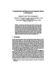
2. 2 Taxonomy of load balancing approaches The load balancing problem is often described in the literature with different terminologies, sometimes even contradictory, making thus the qualitative analysis of the various load balancing approaches difficult. Casavant and Kuhl [6] propose a largely adopted taxonomy, because it is very complete, for scheduling and load balancing algorithms in general purpose distributed computing systems. The organization of the different load balancing schemes is shown in Figure1. Load Balancing Problem

Stati

Dynami Centralized Distribute

Dynami

Global Local

Adaptive

Initiation Sende

Receiver

Non-Adaptive Cooperative

Non-Cooperative

Figure 1: Hierarchical taxonomy for load balancing approaches The elements of Figure1 can be explained as follows: A) Static versus Dynamic - Static load balancing, also known as deterministic distribution, assigns a given job to a fixed resource. Every time the system is restarted, the same binding task resource (allocation of a task to the same resource) is used without considering changes that may occur during the system lifetime. In this approach, every task comprising the application is assigned once to a resource. Thus, the placement of an application is static, and a firm estimate of the computation cost can be made in advance of the actual execution. - Dynamic load balancing takes into account the fact that the system parameters may not be known

beforehand and therefore using a fixed or static scheme will eventually produce poor results. A dynamic strategy is usually executed several times and may reassign a previously scheduled task to a new resource based on the current state of system environment [17]. The advantage of dynamic over static load balancing is that the system needs not be aware of the run-time behaviour of the application before execution. For dynamic strategies, the main problem is how to characterize the exact workload of a system, while it changes in a continuous way (adding and removing computing resources, heterogeneity of the computing resources, bandwidth variations, etc.). Dynamic strategies can be applied both for homogeneous or heterogeneous platforms with different degree of performances. B) Distributed vs. Centralized In dynamic load balancing, the responsibility for making global decisions may lie with one centralized location, or be shared by multiple distributed locations. The centralized strategy has the advantage of ease of implementation, but suffers from the lack of scalability, fault tolerance and the possibility of becoming a performance bottleneck. In distributed strategy, the state of resources is distributed among the nodes that are responsible for managing their own resources or allocating tasks residing in their queues to other nodes. C) Local vs. Global In a local load balancing, each resource polls other resources in its neighbourhood and uses local informations to decide upon a load transfer. However, in a global balancing scheme, global informations of all or part of the system are used to initiate the load balancing. This scheme requires an exchange of workload informations between system elements. D) Cooperative vs. Non-cooperative If a distributed load balancing mode is adopted, the next issue that should be considered is whether the nodes involved in job balancing are working cooperatively or independently. In the noncooperative case, an individual system load balancing acts alone as autonomous entities and make the decisions regarding their own objectives independently of these decisions effects about the rest of the system. E) Adaptive vs. Non adaptive In an adaptive scheme, task migration decisions take into account past and current system performance and are affected by previous decisions or changes in the environment.

Load Balancing Strategy in Grid Environment

In the non-adaptive scheme, parameters used in balancing remain the same regardless the past behaviour of the system. Confusion may arise between dynamic and adaptive balancing. Whereas a dynamic solution takes environmental inputs into account when making its decision, an adaptive solution (which is also dynamic) takes environmental stimuli into account to modify the load balancing policy itself [3]. F) Sender/Receiver/Symmetric Initiated Balancing

Techniques of load balancing tasks in distributed systems have been divided mainly into sender-initiated, receiver-initiated, and symmetrically-initiated [1]. In sender-initiated models, the overloaded resources transfer one or more of their tasks to more under loaded resources. In receiver initiated models, under loaded resources request tasks to be sent to them from resources with higher loads. Finally, in symmetric models, both the under loaded as well as the overloaded resources can initiate load transfer (task migration).

3. RELATED WORKS Research works on load balancing has been focused on system-level load balancing or task scheduling [2, 15]. Their main objective is to maximize the overall throughput or average response time. Most application-level load balancing approaches are oriented on application partitioning via graph algorithms. However, it does not address the issue of reducing migration cost. That is the cost entailed by load redistribution, which can consume order of magnitude more time than the actual computation of a new decomposition. Some works [18] have proposed a latency-tolerant algorithm that takes advantage of overlapping the internal data computation and incoming data communication to reduce data migration cost. Unfortunately, it requires applications to provide such a parallelism between data processing and migration, which restricts its applicability. Payli et al. [16] propose a dynamic load balancing approach to provide application level load balancing for individual parallel jobs in Grid computing environment. Agent-based approaches have been tried to provide load balancing in cluster of machines [5, 14]. In [11] Genaud et al. enhance the MPI_Scatterv primitive to support master-slave load balancing by taking into consideration the optimization of computation and data distribution using a linear programming algorithm. However, this solution is limited to static load balancing. Hu et al. [12] propose an optimal data migration algorithm in diffusive dynamic load balancing through the calculation of Lagrange multiplier of the Euclidean form of transferred weight. This work can effectively minimize the data movement in homogeneous environments, but it does not consider the network heterogeneity. In

particular, workload migration is critical to be considered because the wide area network performance is dynamic, changing throughout execution, instable, etc., in addition to considering the resource heterogeneity. This communication aspect is neglected in traditional application-level load balancing strategies. Scheduling sets of computational tasks on distributed platforms is a key issue but a difficult problem. Although, as mentioned above, a large number of scheduling techniques and heuristics have been presented in the literature, most of them target only homogeneous resources. However, modern computing systems, such as the computational Grid, are most likely to be widely distributed and strongly heterogeneous. Therefore, it is essential to consider the impact of heterogeneity on the design and analysis of scheduling techniques. The traditional objective, when scheduling sets of computational tasks, is to minimize the overall execution time called makespan. However, in the context of heterogeneous distributed platforms, makespan minimization problem is in most cases NP-complete, sometimes even APX-complete [19]. When dealing with large scale systems, an absolute minimization of the total execution time is not the only objective of a load balancing strategy. We think that the communication cost, induced by load redistribution, is also a critical issue. For this purpose, we propose, in this paper, a novel load balancing strategy to address the new challenges in Grid computing. Comparatively to the existing works, the main characteristics of our strategy can be summarized as follows: • It uses a task-level load balancing; • It privileges a local task transfer (within a cluster) more than global transfer (task transfer between clusters); • It reduces tasks moving across the heterogeneous resources of a Grid architecture; • It allows performing more than one load balancing operation at the same time (load balancing operation in each cluster).

4. LOAD BALANCING MODEL 4.1 Grid topology As a topological point of view, we regard a Grid computing as a set of clusters present in a multi-node platform. Each cluster owns a set of worker nodes and belongs to a LAN local domain (Local Area Network). Every cluster is connected to the WAN global network (World Area Network) by a switch. Figure 2 describes this topology.

Journal of Information Technology and Applications Vol. 1 No. 4 March, 2007, pp. 285-296

node node node

Grid Manager

node

Level 0

node node

node Cluster Managers

node

WAN

Level 1

node Level 2

Switch

node node

Clusters

node node

node

LAN

node node

Nodes

Model 1/N

Model 1/N

Model C/N

Figure 2: Example of a Grid topology

4.2 Mapping a Grid into a tree-based model The load balancing strategy proposed in this paper is based on mapping of any Grid architecture into a tree-based model. This tree, illustrated in Figure 3, is built by aggregation as follows: • First, for each cluster we create a two level subtree. The leaves of this sub-tree correspond to the cluster nodes, and its root, called cluster manager, represents a virtual node associated with the cluster. Its role is to manage the cluster workload. • Second, sub-trees corresponding to all clusters are aggregated to generate a three level sub-tree of which root is a virtual node designated as Grid manager. The final tree is denoted by C/N, where C is the number of clusters that compose the Grid and N the number of worker nodes. As illustrated in Figure 3, this tree can be instantiated into two specific trees: C/N and 1/N, depending on the values of C and N. The mapping function generates a non cyclic connected graph where each level has specific functions. • Level 0: In this first level, we have a virtual node called Grid manager, which corresponds to the tree root. This node realizes the following functions: (i) It maintains the workload information of the entire Grid. (ii) It decides to start a global load balancing between the Grid clusters, which we will call an Intra-Grid load balancing. (iii) It sends the load balancing decisions to the nodes of level 1 for execution.

Figure 3: Tree-based representation of a Grid • Level 1: Each virtual node of this level, called cluster manager, is associated with a physical Grid cluster. In our load balancing strategy, this virtual node is responsible for : (i) Maintaining the workload information relating to each one of its worker nodes. (ii) Estimating its associated cluster workload. (iii) Deciding to start a local load balancing, which we will call an Intra-Cluster load balancing. (iv) Sending the load balancing decisions to the worker nodes which it manages. • Level 2: At this last level, we find the worker nodes of the Grid linked to their respective clusters. Each node is responsible for: (i) Maintaining its workload information. (ii) Sending, periodically, this information to its cluster manager. (iii) Performing the load balancing operations decided by its manager.

4.3 Characteristics of the proposed model The proposed model described here is characterized by the following properties: A) It is hierarchical: This propriety will facilitate the flow of workload information through the tree. We distinguish three types of workload information flows: (a) Ascending flow: This flow relates to the workload information flow, to get current workload state.

Load Balancing Strategy in Grid Environment

(b) Horizontal flow: It concerns the useful information (parameters) for the execution of load balancing operations. (c) Descending flow: This flow conveys the load balancing decisions made by the managers corresponding to the various levels of the model. B) It supports Grid heterogeneity and scalability: Connecting or disconnecting resources (worker nodes or clusters) corresponds to simple operations in the tree (adding or removing leaves or sub-trees). C) It is totally independent from any physical Grid architecture: The Grid transformation into a tree is univocal. For each Grid, we can associate one and only one tree, independently of the topological Grid complexity. D) The model C/N is an aggregation of C models 1/N.

5. LOAD BALANCING STRATEGY 5.1 Principles In accordance with the hierarchical structure of the described model, we distinguish between two load balancing levels: Intra-Cluster (inter-nodes) and Intra-Grid (inter-clusters). • Intra-Cluster load balancing: In this first level, depending on its current workload (estimated from workloads of its worker nodes), each cluster manager decides whether to start or not a load balancing operation. If a cluster manager decides to start a load balancing operation, then it tries, in priority, to load balance its workload among its worker nodes. Hence, we can proceed C local load balancing in parallel, where C is the number of clusters. • Intra-Grid load balancing: The load balance at this level is used only if some cluster managers fail to load balance their workload among their associated worker nodes. In this case, tasks of overloaded clusters are transferred to under loaded ones regarding communication cost. The chosen under loaded clusters are those that need minimal communication cost for transferring tasks from overloaded clusters.

use the concept of group and element. Depending on cases, a group designs either a cluster or the Grid (level 1 or level 0 in the tree). An element is a group component (worker node of level 2 or cluster of level 1). The main steps of our strategy can be summarized as follows: A) Step 1: Estimation of the group workload Here we are interested by the information policy to define what information reflects the workload status of the group? When is it to be collected and from where? Knowing the number of available elements under its control and their computing capabilities, each group manager estimates its own capability by performing the following actions: • Estimates its current workload based on workload informations received periodically from its component elements. • Computes the standard deviation over the workload index, in order to measure the deviation between its involved elements. To consider the heterogeneity between nodes capabilities, we propose to take as workload index the processing time1 denoted TEX = LOD SPD . • Sends workload information to its manager. B) Step 2: Decision making In this step, the manager decides whether it is necessary to perform a load balancing operation or not. For this purpose it executes the two following actions: (i) Defining the imbalance/saturation state of the group. If we consider that the standard deviation σ measures the average deviation between the processing times of elements and the processing time of their group, we can say that this group is in balance state when this deviation is small. Indeed, this implies that processing time of each element converges to the processing time of its group. Then, we define the imbalance and saturation states. • Imbalance state: In practice, we define a balance threshold, denoted as ε, from which we can say that the standard deviation tends to zero and hence the group is balanced. We propose for this purpose to define a threshold ε∈[0-1]. Then, we can write the following expression: If (σ ≤ ε) Then the group is Balanced Else it is Imbalanced.

The main advantage of this strategy is to privilege local load balancing in first (within a cluster and then on the entire Grid). The goal of this neighbourhood approach is to decrease the amount of messages between clusters. As a consequence, the communication overhead induced by tasks transfer is reduced.

•

Saturation state: An element can be balanced while being saturated. In this

5.2 Strategy outline At any load balancing level, we propose the following three steps strategy. As the description of this strategy will be done in a generic way, we will

1

We define processing time of an entity (element or group) as the ratio between workload (LOD) and capability (SPD) of this entity.

Journal of Information Technology and Applications Vol. 1 No. 4 March, 2007, pp. 285-296 particular case, it is not useful to start an intra group load balancing since its elements •

will remain overloaded. To measure saturation, we introduce another threshold called saturation threshold, noted as δ. When the current workload of a group borders its capacity, it is obvious that it is useless to balance it since all belonging components are saturated. (ii) Group partitioning. For an imbalance state, we determine the overloaded elements (sources) and the under loaded ones (receivers), depending on the processing time of every element and relatively to processing time of the associated group. C) Step 3: Tasks transfer In order to transfer tasks from overloaded elements to under loaded ones, we propose the following heuristic: (i) Evaluation of the total amount of workload ”Supply”, available on the receiver elements. (ii) Computation of the total amount of workload ”Demand”, required by source elements. (iii) If the supply is much lower than the demand (supply is far to satisfying the request) it is not recommended to start local load balancing. Here, we introduce a third threshold, called expectation threshold denoted as ρ, to measure relative deviation between supply and demand. We can then write the following expression: If (Supply/Demand > ρ) Then perform a Local load balancing Else perform a Higher level load balancing. (iv) Perform the tasks transfer regarding communication cost induced by this transfer and according to the criteria selection of tasks. As criterion selection we propose the following: • Shortest process time which transfer in first the task with shortest remaining processing time. • Longest process time: transfer the task with longest remaining processing time. • FIFO: transfer the first submitted task. • LIFO: transfer the last submitted task. • Random: choosing a task randomly.

5.3 Load Supply and demand estimation The supply of a receiver element Er corresponds to the amount of load Xr that it agrees to receive so that its processing time: TEXr ∈ [TEXG - σG ; TEXG + σG], where σG corresponds to the standard deviation over the processing times of group associated to element Er, and TEXG represents the processing time of this group. In practice, we must reach the convergence:

TEXr Æ TEXG.

TEX r =

LODr + X r LODG ≅ SPDr SPDG

With LOD represents the workload and SPD the capability.

Xr =

LODG .SPDr − LODr SPDG

Thus, we estimate the total supply of receiver set GER by:

Supply =

∑X

E r ∈GER

r

By similar reasoning we determine the demand of a source element Es witch corresponds to the load Ys that it requests to transfer so that: TEXs Æ TEXG.

LODs − Ys LODG ≅ SPDs SPDG LODG .SPDs Ys = LODs − SPDG

TEX s =

The total demand of source set GES is obtained by:

Demand =

∑Y

Es∈GES

s

6. LOAD BALANCING ALGORITHM We define two levels of load balancing algorithms: intra-cluster and intra-Grid load balancing algorithm.

6.1 Intra cluster load balancing algorithm This algorithm is considered as the kernel of our load balancing strategy. The neighbourhood load balancing used by our strategy makes us think that the imbalance situations can be resolved within a cluster. It is triggered when any cluster manager finds that there is a load imbalance between the nodes which are under its control. To do this, the cluster manager receives periodically workload information from each worker node. On the basis of these informations and the estimated balance threshold ε, it analyzes the current workload of the cluster. According to the result of this analysis, it decides whether to start a local balancing in the case of imbalance state, or eventually just to inform its Grid manager about its current workload. At this level, communication costs are not taken into account in the task transfer since the worker

Load Balancing Strategy in Grid Environment

nodes of the same cluster are interconnected by a LAN network, of which communication cost is constant.

6.2 Intra Grid load balancing algorithm This algorithm, that uses a source-initiated approach, performs a global load balancing among all clusters of the Grid. It is started in the extreme case where some cluster managers fail to locally

balance their overload. Knowing the global state of each cluster, the Grid manager can evenly distribute the global overload between its clusters. Contrary to the intra-cluster level, we should consider the communication cost between clusters. A task can be transferred only if the sum of its latency in the source cluster and cost transfer is lower than its latency on the receiver cluster. This assumption will avoid making useless task migration.

6.3 Generic intra-group algorithm (Case of a group G) Step 1: Workload Estimation 1. For Every element Ei of G and according to its specific period Do Sends its workload LODi to its group manager Endfor 2. Upon receiving all elements workloads and according to its period the group manager performs: a- Computes speed SPDG and capacity SATG of G b- Evaluates current load LODG and processing time TEXG of G c- Computes the standard deviation σG over processing times d- Sends workload information of G to its associated manager: in case where G is a cluster Step 2: Decision Making 3. Balance criteria a. Cluster: If (σG ≤ ε ) Then Cluster is balanced; Return EndIf b. Grid: If (# (overloaded clusters)) ≤ given threshold Then Grid is in balance state; Return EndIf 4. Saturation criteria

⎞ ⎛ LODG f δ ⎟⎟ Then Group G is saturated; Return EndIf ⎠ ⎝ SATG

If ⎜⎜

5. Partitioning group G into overloaded (GES), under-loaded (GER) and balanced (GEN) GESÅ Φ; GERÅ Φ; GEN Å Φ For Every element Ei of G Do If ( Ei is saturated) Then GES ÅGES ∪ Ei /* Saturated ⇒ Overloaded */ Else Switch - TEXi > TEXG + σG : GES ÅGES ∪ Ei /* Source */ - TEXi < TEXG - σG : GER ÅGER ∪ Ei /* Receiver */ - TEXG -

σG ≤ TEXi

≤ TEXG +

σG : GEN ÅGEN ∪ Ei

/* Balanced */

EndSwitch EndIf EndFor. Step 3: Tasks Transfer 6. Test on Supply and Demand

Supply =

LODG .SPDr − LODr SPDG E r ∈GER

Demand =

∑

∑

E S ∈GES

Supply If ⎛⎜ ⎝

Demand

LODs −

LODG .SPDs SPDG

≤ ρ ⎞⎟ Then local load balancing Fail; Return EndIf ⎠

7. Perform intra-group task transferring: If (G = Cluster) then Perform Heuristic1 else Perform Heuristic2 EndIf

Journal of Information Technology and Applications Vol. 1 No. 4 March, 2007, pp. 285-296 Heuristic 1: Intra-Cluster tasks transfer a- Sort GES by descending order of their elements processing times. b- Sort GER by ascending order of their elements processing times. c- While (GES ≠ Φ .AND. GER ≠ Φ) Do For i = 1 To # (GER) Do (i) Sort tasks of first node belonging to GES by selection criterion, (ii) Transfer the higher priority task from first source node of GES to ith receiver node of GER (iii) Update the current workloads of receiver and source nodes, (iv) Update sets GES, GER and GEN, (v) If (GES = Φ OR GER =Φ) then Return Endif, (vi) Sort GES by descending order of their processing times. Endfor Done. Heuristic 2: Intra-Grid tasks transfer 1- Sort items of set GES by descending order of their processing times. 2-For Every cluster Cj of GES Do (i) Sort clusters Cr of GER by ascending order of inter-Clusters (Cj-Cr) WAN bandwidth sizes. (ii) Sort nodes of Cj by descending order of their processing times. (iii) While ( GES ≠ Φ AND GER ≠ Φ) Do For i = 1 To # (GER) Do (a) Sort tasks of first node belonging to Cj by selection criterion and communication cost, (b) Transfer the higher priority task from first node of Cj to ith cluster of GER Cr (c) Update the current workloads of Cj and Cr. (d) Update sets GES, GER and GEN. (e) If (GES = Φ OR GER =Φ) Then Return Endif. (f) Sort GES by descending order of their processing times. Endfor Done Endfor

7. EXPERIMENTAL STUDY 7.1 Simulation parameters In order to evaluate the practicability and performance of our proposed strategy, we have developed a Grid simulator in Java. The main parameters used in our experimentations are summarized in the sequel: 1.

2.

Cluster parameters: These parameters give information about worker nodes and clusters such as: Number of nodes and clusters, node capabilities like speeds, capacities and so on. Tasks parameters: These parameters include: (i) Number of tasks queued in each node; (ii) Task submission date; (iii) Number of instructions per task; (iv) Cumulated processing time; (v) Cumulated waiting time.

3.

Network parameters: LAN and various WAN bandwidth sizes.

4.

Performance parameters: In our experimentations we have used three parameters in order to analyze the

performance of the proposed strategy: the number of clusters, their worker nodes and the number of tasks. We have focused on the following objectives relating to a set of tasks submitted during a given period: Average waiting time, Average processing time, Average response time, Average time of communication and Execution time of the load balancing Algorithm. To evaluate the gain obtained by proposed load balancing strategy, we compute the first three metrics in two cases: before (denoted Bef in Table1) and after (Aft) execution of our load balancing algorithms.

7.2 Results All the experiments have been performed on a 3 GHz P4 Intel Pentium with 1 GB main memory, running under Windows XP. In order to obtain reliable results, we have reiterated the same experimentations more than ten (10) times and we have computed the average time. In our experimentations, we consider that the task distribution is done in a periodic and random way according to the uniform law. We randomly generate node capabilities and task parameters. We have set the different thresholds to follows: ε = 0.5;

Load Balancing Strategy in Grid Environment

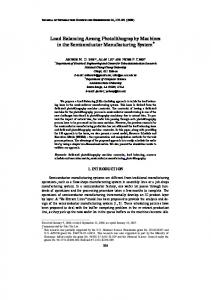
δ = 0.8 and ρ = 0.75. For the selection criterion, we have adopted the shortest process time which transfer in first the task with shortest remaining execution time. This choice is made after the experimentation of several criteria such as first task submitted, last task submitted, random task, task with shortest remaining execution time and task with longest remaining execution time. We highlight in the sequel, only results related to response and communication times, whose we consider as main objective in a load balancing strategy. A) Experiments 1 In the first set of experimentations, we have focused on the response time, the waiting time and the processing time, according to various numbers of tasks and clusters. We have considered different numbers of clusters and we suppose that each cluster contains 50 worker nodes. For every node, we generate a random speed varying between 10 and 30 computing units per time unit. The number of instructions per task has varied between 300 and 1500 computing units. Table 1: Gain realized by proposed strategy #Clusters

3.09% and 24.44%. In more than 60% of cases, this gain is greater than 11%. • The lower gains have been obtained when the number of clusters was fixed at 32 on the one hand and when the number of tasks was 10000 and 20000 on the other hand. We can justify this by the instability of the Grid state (either overloaded or idle). Figure 4 illustrates the gain obtained by the proposed load balancing strategy for various numbers of clusters and tasks. 25

# cluster = 4 # cluster = 8

Gain (%) 20 15

# cluster = 16 # cluster = 32

10 5 0 10000 12000 14000 16000 18000 20000 Number of tasks

4

8

16

32

630 495 21.43%

387 359 07.24%

340 319 6.18%

327 311 4.89%

Figure 4: Gain according to various numbers of clusters by varying the number of tasks

578 509 11.94%

471 413 12.31%

431 380 11.83%

388 376 3.09%

• Best improvements were obtained when the Grid were in a stable state: (for #Clusters ∈{8, 16} and for #Tasks ∈{14000, 16000}.

2099 1776 15.39%

1653 1249 24.44%

1211 987 18.50%

913 809 11.39%

1848 1523 17.59%

1105 911 17.56%

658 502 23.71%

387 310 19.90%

1987 1764 11.22%

1003 932 7.08%

984 831 15.55%

891 823 7.63%

1708 1597 6.50%

1589 1456 8.37%

1211 1077 11.07%

1050 976 7.05%

# Tasks 10000

12000

14000

16000

18000

20000

Bef Aft Gain Bef Aft Gain Bef Aft Gain Bef Aft Gain Bef Aft Gain Bef Aft Gain

Table 1 shows the variation of the average response time (in seconds) before and after execution of our load balancing strategy. We can notice the following: • Our strategy has allowed to reduce in a very clear way the mean response time of the tasks. We obtain a gain in 100% of cases, varying between

• In some infrequent cases, we have noted that the variation of the gain changes abruptly. We believe that this situation comes from the fact that the number of tasks and/or the number of clusters varies suddenly and generates instability in the Grid. B) Experiments 2 For this second set of experimentations we have been interested in the average communication time. Results of the experiments related to this metric are gathered in Figures 5 and 6.

20000

18000

16000

12000

450 400 350 300 250 200 150 100 50 0

14000

# cluster = 4 # cluster = 8 # cluster = 16 # cluster = 32

10000

Average communication time (sec)

Journal of Information Technology and Applications Vol. 1 No. 4 March, 2007, pp. 285-296

Number of Tasks

Average communication time (sec)

Figure 5: Variation of communication time with number of tasks

450 400 350

10000

300

12000 14000

250

16000

200

18000

150

20000

100 50 0 4

8

16

32 Number of clusters

Figure 6: Variation of communication time with number of clusters The variation of this metric is very sensitive to the initial distribution of the tasks and to the disparity between node capabilities (when some nodes have a high speed while others have very low capabilities). In Figure 5, we remark that the minimum is reached for 16000 tasks and 32 clusters. This result justifies the 19.9% of gain obtained for the response time. It is explained by the fact that the random distribution of tasks has been rather equitable. For a number of tasks equal to 20000, the curve associated with a number of clusters equal to 4 has reached its maximum. Indeed, for this value and to reach a load balancing, it is necessary to transfer more tasks because of their random distribution. Figure 6 lets us think that the average communication time is linearly proportional to the number of tasks. 7 CONCLUSION This paper has addressed the problem of load balancing in Grid computing. We have proposed a

load balancing strategy based on a tree representation of a Grid. The model takes into account the heterogeneity of resources and it is completely independent from any physical Grid architecture. Our proposal load balancing strategy privileges local load balancing in first (load balance within clusters without WAN communication). Considering the overhead generated by the execution of load balancing system, our strategy starts a balancing operation only when it ensures that it is efficiency. To validate the proposed strategy, we have developed a Grid simulator in order to measure its performance. The first experimentation results are very promising and lead to a better load balancing between nodes of a Grid without high computing overhead. We have obtained good results especially for the average response time of tasks. In the future, we plan to integrate our load balancing strategy on known simulators in the field of Grids, such as GridSim. This will allow us to measure the effectiveness of our strategy in the existing simulators. We also intend to integrate our strategy as a service of GLOBUS middleware.

REFERENCES [1] M. Arora, S.K. Das and R. Biswas. ‘A decentralized scheduling and load balancing algorithm for heterogeneous Grid environments’, Workshop on Scheduling and Resource Management for Cluster Computing, Vancouver, Canada, pp. 499-505, August 2002. [2] C. Banino, O. Beaumont, A. Legrand and Y. Robert, Scheduling strategies for master-slave tasking on heterogeneous processor Grids, Applied Parallel Computing: Advanced Scientific Computing: 6th International Conference (PARA’02), Lecture Notes in Computer Science, vol. 2367, pp. 423–432 Springer-Verlag, 2002. [3] F. Berman, G. Fox and Y. Hey. Grid Computing: Making the Global Infrastructure a Reality. Wiley Series in Communications Networking & Distributed Systems, 2003. [4] R. Buyya, D. Abramson, J. Giddy and H. Stockinger. ‘Economic models for resource management and scheduling in Grid computing’, Journal of Concurrency and Computation: Practice and Experience, 14(13-15): pp.1507-1542, December 2002. [5] J. Cao, Daniel P. Spooner, Stephen A. Jarvis, S. Saini and Graham R. Nudd. Agent-Based Grid Load Balancing Using Performance-Driven Task Scheduling.: Proceedings of the 17th International Symposium on Parallel and Distributed Processing, pages 49.2, 2003.

Load Balancing Strategy in Grid Environment

[6]

T.L. Casavant and J.G. Khul. ‘A taxonomy of scheduling in general purpose distributed computing systems’. IEEE Transactions on Soft. Engineering, 14(2):pp.141-153, 1994.

[7] A. Chervenak, I. Foster, C. Kesselman, C.Salisbury and S.Tuecke. ‘The data Grid: towards an architecture for the distributed management and analysis of large scientific datasets. Journal of Network and Computer Applications, 23(3):pp.187-200, 2000. [8] I. Foster and C. Kesselman (editors). ‘The Grid: Blueprint for a Future Computing Infrastructure’, Morgan Kaufmann, USA, 1999. [9] I. Foster, C. Kesselman, J.M. Nick, and S. Tuecke. ‚Grid services for distributed system integration’. IEEE Computer, 35(6):pp.37-46, 2002. [10] I. Foster, C. Kesselman, and S. Tuecke. ‘The anatomy of the Grid: Enabling scalable virtual organizations’. Internal Journal of High Performance Computing Applications, 15(3), 2001. [11] S. Genaud, A. Giersch and F. Vivien. ‘Load balancing scatter operations for Grid computing’, 12th Heterogeneous Computing Workshop, IEEE CS Press, 2003. [12] Y.F. Hu, R.J. Blake, and D.R. Emerson. ‘An optimal migration algorithm for dynamic load balancing’, Concurrency: Practice and Experience, 10:pp.467-483, 1998. [13] K.Y. Kabalan, W.W. Smar and J.Y. Hakimian. ‘Adaptive load sharing in heterogeneous systems: policies, modifications and

simulation’. Int. Journ. of SIMULATION, 3(12):pp.89-100, 2002. [14] C. C. Myint and K.M. Lar Tun. ‘A Framework of Using Mobile Agent to Achieve Efficient Load Balancing in Cluster’, 6th Asia-Pacific Symposium on Information and Telecommunication Technologies, APSITT2005, pp 66-70, Nov 9-10, 2005; Yangon, Myanmar. [15] A. Olugbile, H. Xia, X. Liu and A. Chien. ‘New Grid Scheduling and Rescheduling Methods in the GrADS Project’, Workshop for Next Generation Software, Santa Fe, New Mexico, April 2004, held in conjunction with the IPDPS 2004. [16] R.U. Payli, E. Yilmaz, A. Ecer, H.U. Akay and S. Chien. ‘DLB: A Dynamic Load Balancing Tool for Grid Computing’, Parallel CFD Conference, May 24-27, 2004, Grand Canaria, Canary Islands, Spain. [17] H. G. Rotithor. ’Taxonomy of dynamic task scheduling schemes in distributed computing systems’, IEE Proceedings on Computer and Digital Techniques, 141 (1), pp. 1–10, 1994. [18] H. Shan, L. Oliker, R. Biswas, and W. Smith. ’Scheduling in heterogeneous Grid environments: The effects of data migration’. In Proc. of ADCOM2004: International Conference on Advanced Computing and Communication, India, December 2004. [19] C.Z. Xu and F.C.M. Lau. ‘Load Balancing in Parallel Computers: Theory and Practice’. Kluwer, Boston, MA, 1997.